
Deep Neural Networks (DNNs) have become very successful in the domain of artificial intelligence. They have begun to directly influence our lives through image recognition, automated machine translation, precision medicine and many other solutions. Furthermore, there are many parallels between these modern artificial algorithms and biological brains: The two systems resemble each other in their function - for example, they can solve surprisingly complex tasks - and in their anatomical structure - for example, they contain many hierarchically structured neurons.
Given these apparent similarities, many questions arise: How similar are human and machine vision really? Can we understand human vision by studying machine vision? Or the other way round: Can we gain insights from human vision to improve machine vision? All these questions motivate the comparison of these two intriguing systems.
While comparison studies can advance our understanding, they are not straightforward to conduct. Differences between the two systems can complicate the endeavor and open up several challenges. Therefore, it is important to carefully investigate the comparisons of DNNs and humans.
In our recently published preprint “The Notorious Difficulty of Comparing Human and Machine Perception”, we highlight three of the most common pitfalls that can easily lead to fragile conclusions:
- Humans can be too quick to conclude that machines learned human-like concepts. This is similar to our tendency of quickly concluding that an animal would be happy or sad, simply because its face might have a human-like expression.
- It can be tricky to draw general conclusions that reach beyond the tested architectures and training procedures.
- When comparing humans and machines, experimental conditions should be equivalent.
Pitfall 1: Humans are often too quick to conclude that machines learned human-like concepts
Let’s start with a small experiment on yourself: Does the following image contain a closed contour?
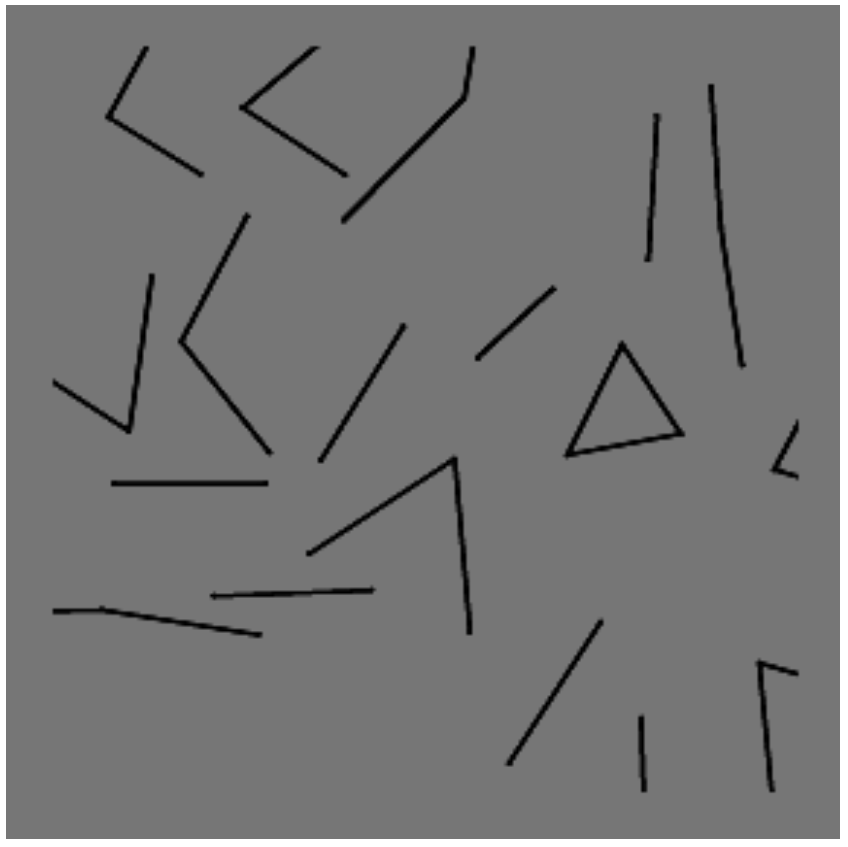
And how about this image?

It was probably very easy for you to determine that both images had a closed contour. According to Gestalt theory, the perception of closure is thought to be an important component of how the human visual system derives meaning from the world. The process is often called “contour integration”: To tell if a line closes up to form a closed contour, humans can use global information - as local regions of an image are not sufficient to provide a complete story.
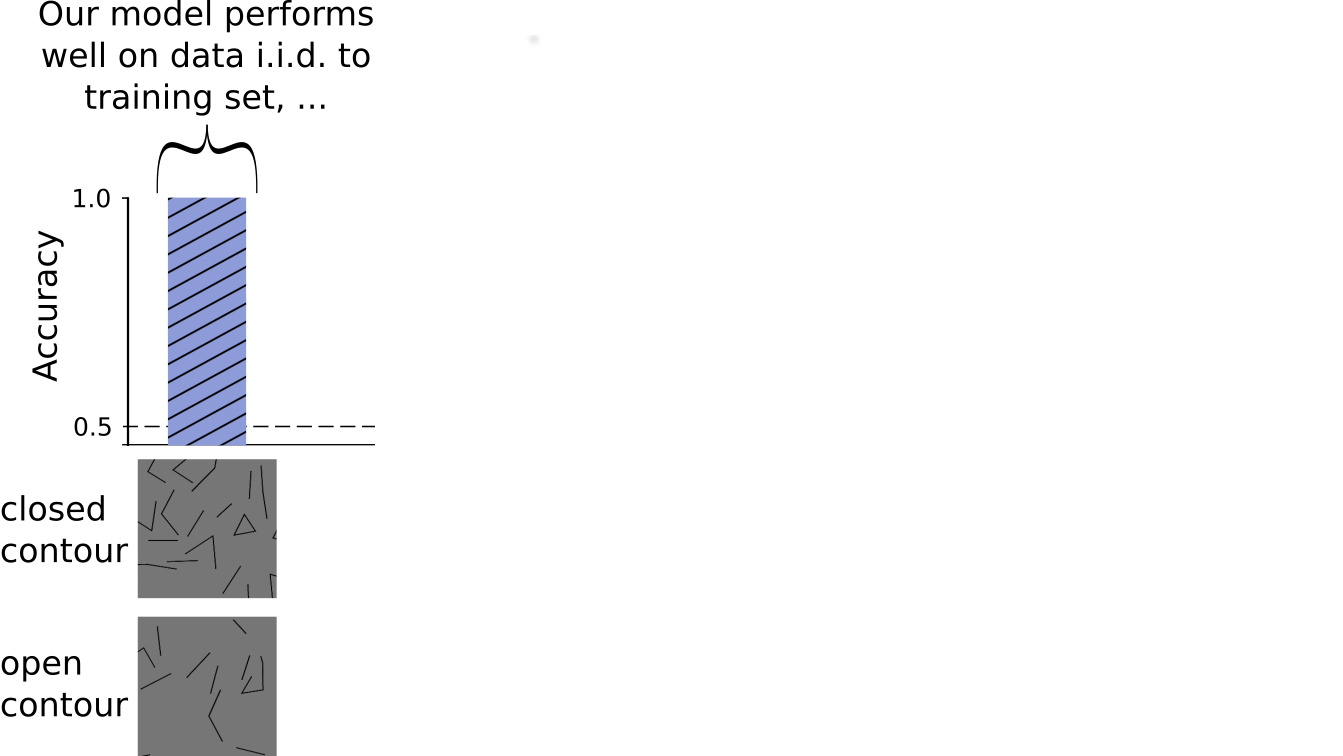
We hypothesized that convolutional neural networks would struggle at global contour integration. By their nature, convolutions process a lot of local information in most of their layers and have relatively little capacity to process global information, leading them to prefer texture over shape in object recognition (e.g. Geirhos et al. (2018), Brendel and Bethge (2019)). We trained the network on the following set of images with closed and open contours:

Surprisingly, the trained model performed this task almost perfectly: it could easily distinguish whether an image contained a closed contour. This is shown in the graph below. The y-axis shows accuracy, which is a measure of the fraction of correct predictions. A value of 1 means that the model predicted all images correctly, whereas 0.5 corresponds to chance performance.
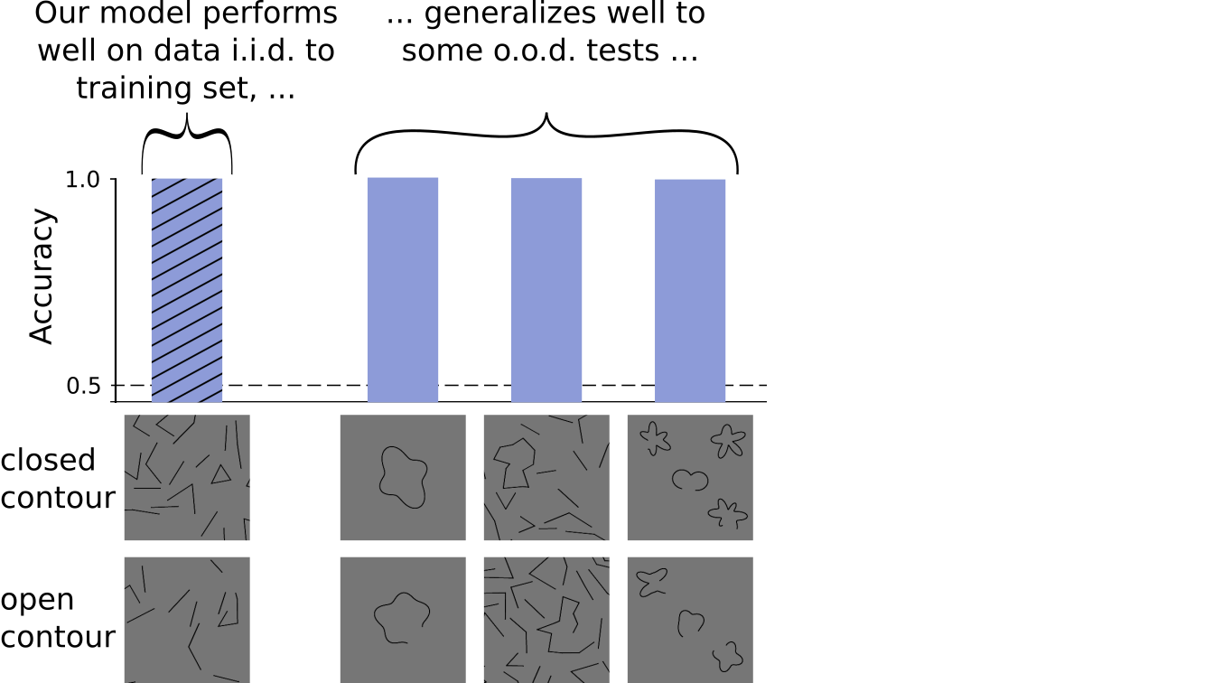
Does this mean DNNs effortlessly perform global contour integration like humans? If this were the case, the model should be able to work well on variations of the dataset without any further training on the new images.
Following this logic, we proceeded with testing our model’s performance on a sample of out-of-distribution (o.o.d.) images: Unlike in the original data set, the main contours now consisted of, for example, more edges, or the straight lines became curvy ones. This test should reveal if our model just picked up some other statistical cues in the original images (e.g. maybe the number of black or white pixels differed for closed vs. open images etc), or if it really understood the concept of closedness.
Again, we were surprised to see that our model performed well on the new images or in other words, our model generalized well.
From this data, we could have concluded that DNNs would be able to learn “closedness” as an abstract concept. However, this was not the full story yet. We looked at a few more variations of the dataset. This time, we varied the color or thickness of the lines. For these new images, our model was not able to predict whether an image contained a closed contour. Its accuracy dropped to almost 50% - which corresponds to a random guess.

The failure on these new images showed that the DNN’s strategy did not work on all variations of the data set. A natural follow-up question was what strategy the model might have learned.
As we hypothesized in the beginning, it appears that global information would be required to perform our task well. To test this, we used a network which had access to local regions only (Brendel & Bethge, 2019). Interestingly, we found that the DNN continued to perform well even when the patches that were fed to this network were smaller than the closed contours. This finding suggested that global information was not required to detect closedness in our set of stimuli. The following figure illustrates the local features that could be used: The length of certain lines provided evidence for the correct class.

As humans, we often have a bias regarding how a specific task is solved. In our case, we thought the only way to solve closed contour detection would be by contour integration. This hypothesis turned out to be incorrect. Instead, there was a simple solution based on local features - which, from a human perspective, was difficult to anticipate.
When comparing humans and machines, it is important to remember that DNNs can find solutions that differ fundamentally from the ones we expect them to use. To avoid drawing premature and human-biased conclusions, it is important to thoroughly examine the model, its decision-making process and the data set.
Pitfall 2: Drawing general conclusions that reach beyond the tested architectures and training procedures is tricky.
The following figure shows two examples of the Synthetic Visual Reasoning Test (SVRT) (Fleuret et al., 2011). Can you solve them?

Each of the 23 problems in the SVRT data set can be assigned to one of two task categories. The first category is called "same-different tasks" and requires the judgment of whether shapes are identical. The second category is called "spatial tasks" and requires a decision based on the spatial arrangement of shapes, for example, whether a shape is in the center of another shape.
Humans are typically very good at SVRT problems. They need only a few example images to learn the underlying rule and are then able to correctly classify new images (Fleuret et al., 2011).
Two research groups [Stabinger et al. (2016) and Kim et al. (2018)] tested deep neural networks on the SVRT data set. They found a strong difference between task categories: Their models could perform well on spatial tasks, but not on same-different tasks. Kim et al. (2018) suggested that the feedback mechanisms in the human brain, such as recurrent connectivity, would be important for same-different tasks.
These results have been cited with the broader claim that DNNs in general would not be able to perform well on same-different tasks. Our experiments presented below provide evidence that this is not the case.
The DNNs used by Kim et al. (2018) consisted only of 2-6 layers. The DNNs that are commonly used for tasks such as object classification are much larger. We wanted to know if similar results would be found with standard DNNs. For this reason, we performed the same experiment using ResNet-50 (He, et al., 2016).
Interestingly, we found that ResNet-50 reached accuracies above 90 percent for all tasks, including same-different tasks, even with much fewer training images compared to Kim et al. (28000 instead of 1 million). This finding shows that feed-forward DNNs can indeed reach high accuracies on same-different tasks.

In a second experiment we used only 1000 training samples. In this scenario, we found that for most spatial tasks, high accuracies could still be reached, while the accuracy dropped for same-different tasks. Does this mean that same-different tasks are more difficult? We argue that the low data regime is not a meaningful test for task difficulty. The learning speed greatly depends on the starting condition of a system. In contrast to our DNNs, humans profit from life-long learning. In other words, it might very well be that a human visual system trained from scratch on the two categories of tasks would exhibit a similar difference in sample efficiency as a ResNet-50.
What did we learn from this case study for the comparison of human and machine vision? First, one needs to be careful when making statements about DNNs not being able to perform well on a specific task. Training DNNs is complex and their performance depends strongly on the tested architectures and aspects of the training procedure. Secondly, it is important to remember that DNNs and humans have different starting conditions. Thus one needs to be careful when drawing conclusions from settings where little training data is used.
To summarize, care has to be taken when drawing general conclusions that reach beyond the tested architectures and training procedures.
Pitfall 3: When comparing humans and machines, experimental conditions should be equivalent
Look at the left photo in the figure below. It is pretty obvious that you see a pair of glasses, isn’t it? If we now crop the photo a bit, the object is still clear. We can keep doing this for a few more times and we will still be able to recognize the pair of glasses. However, at some point, this will change: we cannot recognize the object anymore.
The interesting aspect of this transition from a recognizable to an unrecognizable crop is its sharpness: The slightly larger crop (which we call the “minimal recognizable crop”) is classified correctly by most people (e.g. 90%), while the slightly smaller crop (the “maximal unrecognizable crop”) is classified correctly by few people (e.g. 20%). The drop in recognizability is called the “recognition gap” (Ullman et al., 2016). It is computed by subtracting the proportion of people who correctly classified the maximally unrecognizable crop from that of the people who correctly classified the minimal recognizable crop. In the figure below, the recognition gap evaluates as 0.9 - 0.2 = 0.7.

Having found the minimal part of the image for which humans could still identify an object, Ullman et al. (2016) also tested machines: Would machine vision algorithms have a similarly pronounced gap? They found that the recognition gap was much smaller in the tested machine vision algorithms (namely 0.14) and concluded that machine vision systems would function differently (compare the two left bars in the figure after the next one).
In our work, we revisited the recognition gap in a very similar experimental design but with one crucial difference: instead of testing machines on human-selected patches, we tested them on machine-selected patches. Specifically, we implemented a search algorithm with a state-of-the-art deep convolutional neural network that mimicked the human experiment. This ensured that machines were evaluated on patches they selected - just like humans were evaluated on patches they selected.

We found that under these conditions our neural network did experience a similarly large recognition gap between minimal recognizable and maximal unrecognizable crops - just as identified for humans by Ullman et al. (2016).

This case study illustrates that appropriately aligned testing conditions for both humans and machines are essential to compare phenomena between the two systems.
Conclusions
Our three case studies highlight several difficulties when comparing humans and machines. Particularly, we illustrated that confirmation bias can lead to misinterpreting results, that generalizing conclusions from specific architectures and training procedures is tricky, and that unequal testing procedures can confound decision behaviors. In summary, we showed that care must be taken to perform comparisons rigorously and minimize our natural human bias. Only then can comparison studies between AI and humans be fruitful.
Author Bio
Christina and Judy are both grad students at the University of Tübingen and aim to improve understanding visual perception by connecting state-of-the-art object recognition algorithms and the human visual system. They work in the lab of Prof. Dr. Matthias Bethge and belong to the International Max Planck Research School for Intelligent Systems.
Acknowledgments
This post was written by Christina Funke and Judy Borowski with steady support from Wieland Brendel. Great feedback was integrated from Karolina Stosio, Tom S. A. Wallis, Robert Geirhos and Matthias Kümmerer as well as editors from The Gradient: Kiran Vaidhya and Andrey Kurenkov.
Human and machine illustration taken from https://www.flickr.com/photos/gleonhard/33661762360 under the license https://creativecommons.org/licenses/by-sa/2.0/
Citation
For attribution in academic contexts or books, please cite this work as
Judy Borowski and Christina Funke, "Challenges of Comparing Human and Machine Perception", The Gradient, 2020.
BibTeX citation:
@article{borowski2020challengs,
author = {Borowski, Judy and Funke, Christina},
title = {Challenges of Comparing Human and Machine Perception},
journal = {The Gradient},
year = {2020},
howpublished = {\url{https://thegradient.pub/challenges-of-comparing-human-and-machine-perception/ } },
}
If you enjoyed this piece and want to hear more, subscribe to the Gradient and follow us on Twitter.
