
Image recognition (i.e. classifying what object is shown in an image) is a core task in computer vision, as it enables various downstream applications (automatically tagging photos, assisting visually impaired people, etc.), and has become a standard task on which to benchmark machine learning (ML) algorithms. Deep learning (DL) algorithms have, over the past decade, emerged as the most competitive image recognition algorithms; however, they are by default “black box” algorithms: it is difficult to explain why they make a specific prediction.
Why is that an issue? Users of ML models often want the ability to interpret which parts of the image led to the algorithm’s prediction for many reasons:
- Machine learning developers can analyze interpretations to debug models, identify biases, and predict whether the model is likely to generalize to new images
- Users of machine learning models may trust a model more if provided explanations for why a specific prediction was made
- Regulations around ML such as GDPR require some algorithmic decisions to be explainable in human terms
Motivated by these use cases, during the last decade, researchers developed many different methods to open the “black box” of deep learning, aiming to make underlying models more explainable. Some methods are specific for certain kinds of algorithms, while some are general. Some are fast, and some are slow.
In this piece, we provide an overview of the interpretation methods invented for image recognition, discuss their tradeoffs and provide examples and code to try them out yourself using Gradio.
Leave-One-Out
Before we dig into the research, let’s start with a very basic algorithm that works for any type of image classification: leave-one-out (LOO).
LOO is an easy method to understand; it’s the first algorithm you might come up with if you were to design an interpretation method from scratch. The idea is to first segment the input image into a bunch of smaller subregions. Then, you run a series of predictions, each time masking (i.e. setting the pixel values to zero of) one of the subregions. Each region is assigned an importance score based on how much its “being masked” affected the prediction relative to the original image. Intuitively, these scores quantify which regions are most responsible for the prediction.
So if we segment our image into 9 subregions in a 3x3 grid, here’s what LOO would look like:

The darkest red squares are the ones that most changed the output, whereas the lightest had the least effect. In this case, when the top-center region was masked, the prediction confidence dropped the most, from an initial 95% to 67%.
If we segment in a better way (for example, using superpixels instead of grids), we get a pretty reasonable saliency map, which highlights the face, ears and tail of the doberman.

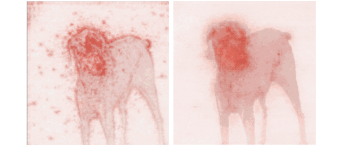
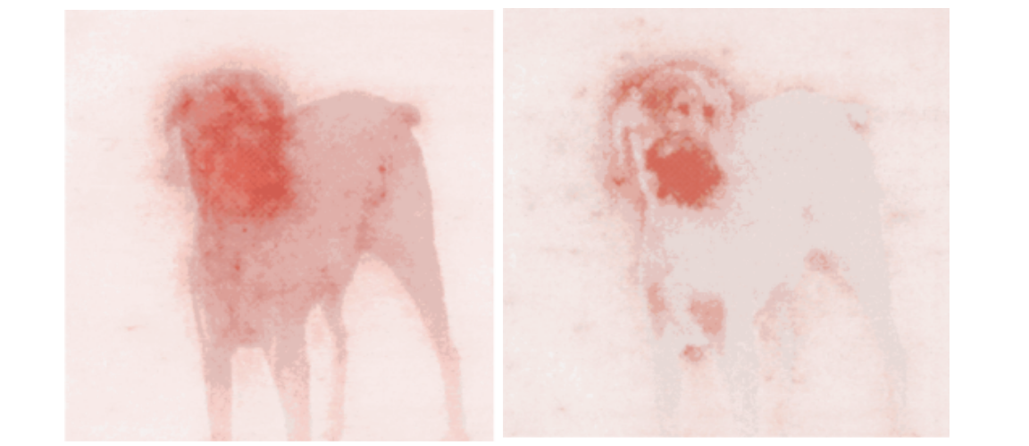
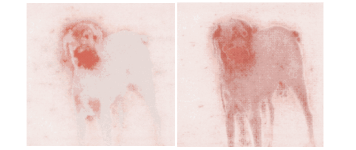
LOO is a simple yet powerful method. Depending on the image resolution and how the segmentation is done, it can generate very accurate and useful results. Here is LOO applied to a 1100 × 825 image of a Golden Retriever as predicted using InceptionNet.
One huge advantage of LOO in practice is that it doesn’t need any access to the internals of the model and can even work on other computer vision tasks besides recognition, making it a flexible all-purpose-tool.
So what are the drawbacks? First, it’s slow. Every time a region is masked, we run inference on the image. To get a saliency map with reasonable resolution, your mask size might have to be small. So, if you segment the image into 100 regions, it will take 100x the inference time to get the heat map. On the other hand, if you have too many subregions, masking any one of them will not necessarily produce a big difference in the prediction. This LOO’s second limitation, which is that it does not take into account interdependencies between regions.
So, let’s look at a much faster and slightly more involved technique: (vanilla) gradient ascent.
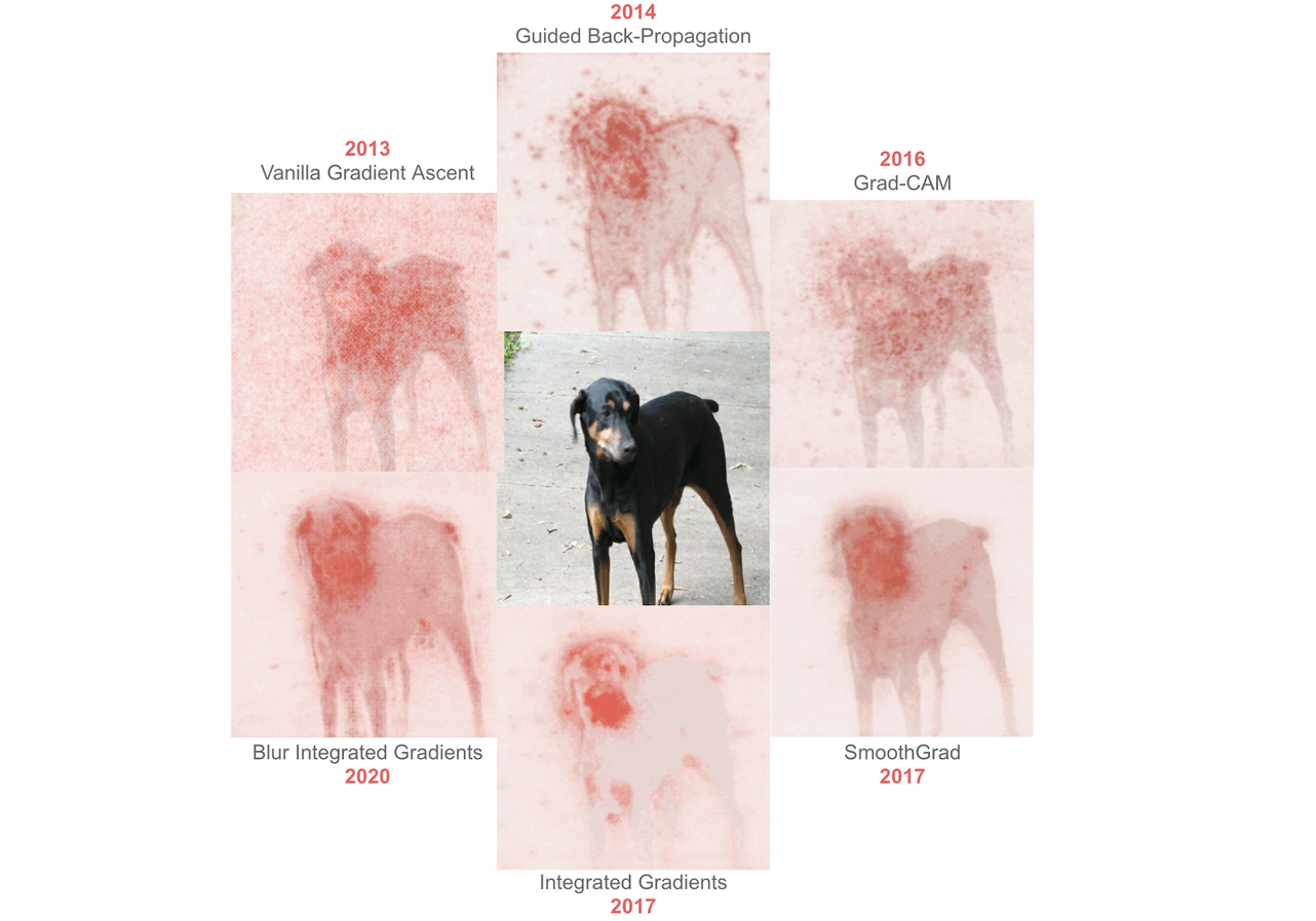
Vanilla Gradient Ascent [2013]

(Vanilla) gradient ascent was presented in the Visualizing Image Classification Models and Saliency Maps [2013] paper. There is a conceptual relationship between LOO and gradient ascent. With LOO, we considered how the output changed when we masked each region in the image, one by one. With gradient ascent, we calculate how the output is affected by each individual pixel, all at once. How do we do this? With a modified version of backpropagation.
With standard back-propagation, we compute the gradient of the model’s loss with respect to the weights. The gradient is a vector that contains a value for each weight, reflecting how much a small change in that weight will affect the output, essentially telling us which weights are most important for the loss. By taking the negative of this gradient, we minimize the loss during training. For gradient ascent, we instead take the gradient of the class score with respect to the input pixels, telling us which input pixels are most important in classifying the image. This single step through the network gives us an importance value for each pixel, which we display in the form of a heatmap, like shown below.
Here’s what that would look like for our Doberman image:

The main advantage here is speed; because we only need to make one pass through the network, gradient ascent is much faster than LOO, although the resulting heatmap is a little grainy.
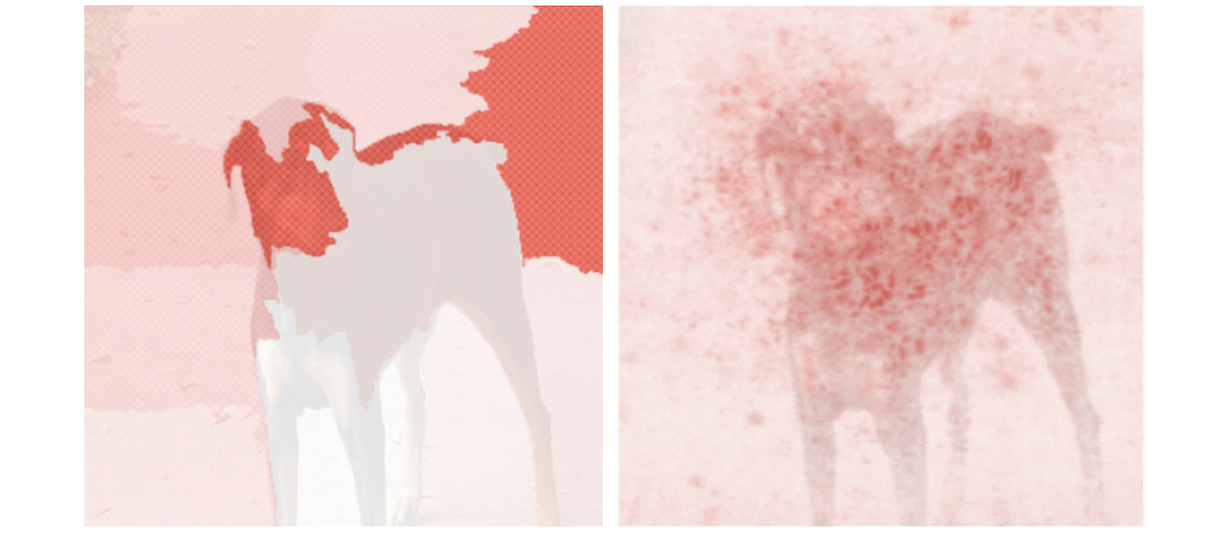
Although gradient ascent works, it was discovered that this original formulation, called vanilla gradient ascent, has a significant shortcoming: it propagates negative gradients, which end up causing interference and a noisy output. A new method, “guided backpropagation,” was proposed to fix these issues.
Guided Back-Propogation [2014]
Guided back-propagation was published in Striving for Simplicity: The All Convolutional Net [2014], where the authors proposed adding an additional guidance signal from the higher layers to the usual step of back-propagation. In essence, the method blocks the backward flow of gradients from neurons whenever the output is negative, leaving only those gradients that result in increased output, which ultimately results in a less noisy interpretation.
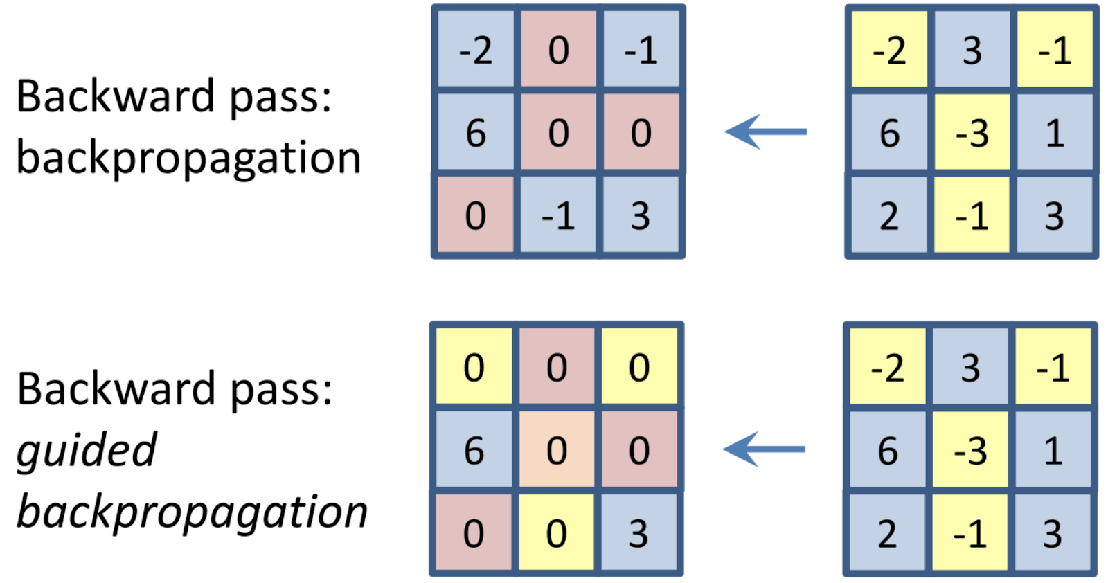
Guided back-propagation works about as fast as vanilla gradient ascent, since it only requires one pass through the network, but usually produces a cleaner output, especially around the edges of the object. The method works particularly well relative to other methods in neural architectures that don’t have max-pooling layers.
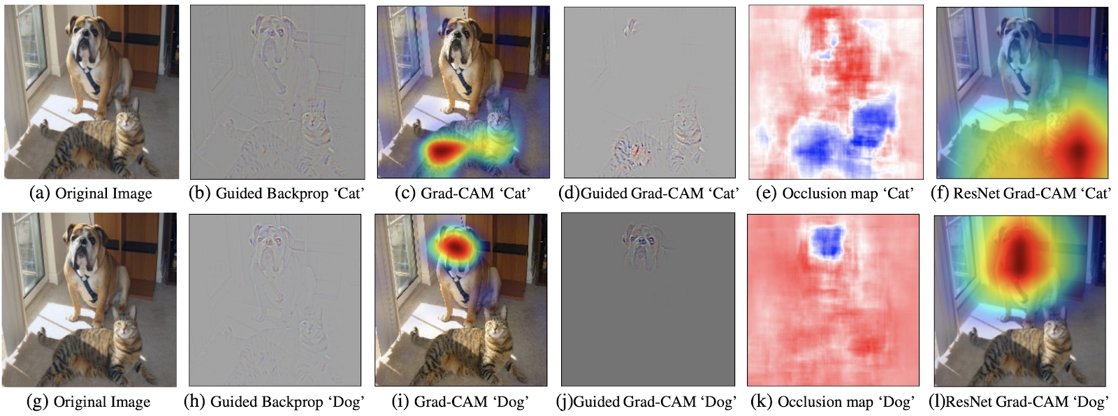
However, it was discovered that there is still a major issue with vanilla gradient ascent and guided back-propagation: they don’t work so well when there are two or more classes present in the image, which often occurs with natural images.
Grad-CAM [2016]
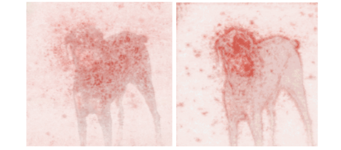
Enter Grad-CAM, or Gradient-Weighted Class Activation Mapping, presented in Grad-CAM: Visual Explanations from Deep Networks via Gradient-based Localization [2016]. Here the authors found that the quality of interpretations improved when the gradients were taken at each filter of the last convolutional layer, instead of at the class score (but still with respect to the input pixels). To get a class-specific interpretation, Grad-CAM does a weighted average of these gradients, with the weight based on a filter’s contribution to the class score. The result, as shown below, is far better than guided back-propagation alone.
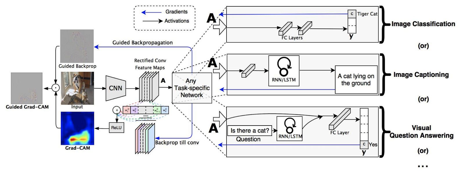
The authors further generalized Grad-CAM to work not just with a target class, but with any target “concept.” This meant that Grad-CAM could be used to interpret why an image captioning model predicted a particular caption, or even handle models that take several inputs, like a visual question-answering model. As a result of this flexibility, Grad-CAM has become quite popular. Below is an overview of its architecture.
SmoothGrad [2017]
Yet, you may have noticed that with all the previous methods, the results are still not very sharp. SmoothGrad, presented in SmoothGrad: removing noise by adding noise [2017]], is a modification of previous methods. The idea is quite simple: the authors noted that if the input image is first perturbed with noise, you can compute gradients once for each version of the perturbed input and then average the sensitivity maps together. This leads to a much sharper result, albeit with a longer runtime.
Here’s how Guided Back-Propagation looks next to SmoothGrad:
When you’re faced with all of these interpretation methods, which one do you choose? Or when methods conflict, is there one method that can be proven theoretically to be better than the others? Let’s look at integrated gradients.
Integrated Gradients [2017]
Unlike previous papers, the authors of Axiomatic Attribution for Deep Networks [2017] start from a theoretical basis of interpretation. They focus on two axioms: sensitivity and implementation invariance, that they posit a good interpretation method should satisfy.
The Axiom of Sensitivity means that if two images differ in exactly one pixel (yet have all of the other pixels in common), and produce different predictions, the interpretation algorithm should give non-zero attribution to that different pixel. The Axiom of Implementation Invariance means that the underlying implementation of the algorithm should not affect the result of the interpretation method. They use these principles to guide the design of a new attribution method called Integrated Gradients (IG).
IG begins with a baseline image (usually a completely darkened version of the input image), and increases the brightness until the original image is recovered. The gradients of the class scores with respect to the input pixels are computed for each image and are averaged to get a global importance value for each pixel. Beyond the theoretical properties, IG thereby also solves another problem with vanilla gradient ascent: saturated gradients. Because gradients are local, they don’t capture the global importance of pixels, only the sensitivity at a particular input point. By varying the brightness of the image and computing the gradients at different points, IG is able to get a more complete picture of the importance of each pixel.
Although this usually produces more accurate sensitivity maps, the method is slower and introduces two new additional hyperparameters: the choice of baseline image and the number of steps over which to produce the integrated gradients. Can we do without these?
Blur Integrated Gradients [2020]

That’s what our final interpretation method, blur integrated gradients seeks to do. Presented in Attribution in Scale and Space [2020], the method was proposed to solve specific issues with integrated gradients, including the elimination of the ‘baseline’ parameter, and removing certain visual artifacts that tend to appear in interpretations.
The blur integrated gradients method works by measuring gradients along a series of increasingly blurry versions of the original input image (rather than dimmed versions of the image, as integrated gradients does). Although this may seem like a minor difference, the authors argue that this choice is more theoretically justified, as blurring an image cannot introduce new artifacts into the interpretation, in the way that choosing a baseline image can.
Final Words
The 2010s were a fruitful decade for interpretation methods for machine learning, and a rich suite of methods now exist that explain neural network behavior. We’ve compared them in this blog post, and we are indebted to several awesome libraries, particularly Gradio to create the interfaces that you see in the GIFs and PAIR-code’s TensorFlow implementation of the papers. The model used for all of the interfaces is the Inception Net image classifier.
Complete code to reproduce this blog post can be found on this Jupyter notebook and on Google Colab. Try out the live interface (with guided back-propagation) here.

Author Bio
Ali is a co-founder of Gradio, where he works as a machine learning engineer. Before that, he spent time at Tesla, iRobot and MIT. He published several academic papers, and has contributed to many open-source projects. You can find him on twitter @si3luwa.
Acknowledgements
Thanks to Andrey Kurenkov, Abubakar Abid and Jessica Dai for their immense help in putting this piece together.
Citation
For attribution in academic contexts or books, please cite this work as
Ali Abdalla, "A Visual History of Interpretation for Image Recognition", The Gradient, 2021.
BibTeX citation:
@article{abid2021visual,
author = {Abdalla, Ali},
title = {A Visual History of Interpretation for Image Recognition},
journal = {The Gradient},
year = {2021},
howpublished = {\url{https://thegradient.pub/a-visual-history-of-interpretation-for-image-recognition/} },
}
If you enjoyed this piece and want to hear more, subscribe to the Gradient and follow us on Twitter.