This is an updated version of a piece originally posted on the author’s blog.
Released in 2018, BERT has quickly become one of the most popular models for natural language processing, with the original paper accumulating tens of thousands of citations. Its success recipe lies in a simple training method called masked language modeling. Randomly mask ~15% of the words in a text, and then ask the model to recover these based on the surrounding context. This simple idea, scaled on billions of words, allowed BERT to develop a deep understanding of human language, reusable for other tasks such as question answering, text summarization, classification of text documents, etc. Given the impressive success of BERT for written language, it is no surprise that researchers are attempting to apply the same recipe to other modalities of language, like human speech.
Could we replace the text input in BERT with a speech sequence, mask a part of it, and similarly train the model to recover what is missing?
Unfortunately, it is not as straightforward as one might assume. Written language can be naturally broken down into words (or sub-words) from a finite vocabulary of discrete units. Speech, originally a sound wave, is recorded as a sequence of continuous values and does not show such natural sub-units. In theory, we could use phonetic systems like phones to discretize speech, but this would first require humans to label the entire dataset beforehand preventing us from pre-training on a large quantity of unlabeled data as BERT does.
In this article, we will introduce the wav2vec 2.0 and HuBERT models. They both offer different solutions to the above problem. They both:
- Transform the original continuous acoustic data into a sequence of discrete units.
- Mask a random part of the sequence and train the model to recover it.
- Use a BERT-like Transformer encoder to model the context of the speech sequence.
However, they do these things in widely different ways. We will look at both models in detail to understand all the subtleties and design choices that come into play when applying a BERT-like approach to speech or acoustic data.
Wav2vec 2.0
This model from Meta AI is a sequel to the first version, originally made of two large convolutional networks called the encoder and context network. Version 2.0 replaces the context network with the Transformer-based BERT architecture. The core idea behind wav2vec 2.0 is to teach the model to do two things in parallel:
- Quantize continuous speech data into discrete units automatically.
- Guess the correct discrete units (learned from step 1) at randomly masked locations.
The challenge of doing these two things together is how to prevent the model from cheating. Since the model both chooses the ground truth targets (step 1) and guesses these targets (step 2), it could collapse into a naive approach without learning anything about the structure of spoken language. For example, the model could assign the same target to every part of the speech sequence, and then always predict this target. Wav2vec 2.0 introduces a set of tactics to mitigate this risk. One of these replaces BERT’s original cross-entropy loss with a contrastive loss. We will look into the details of the training loss, but first, let’s take a step back and look at the big picture.

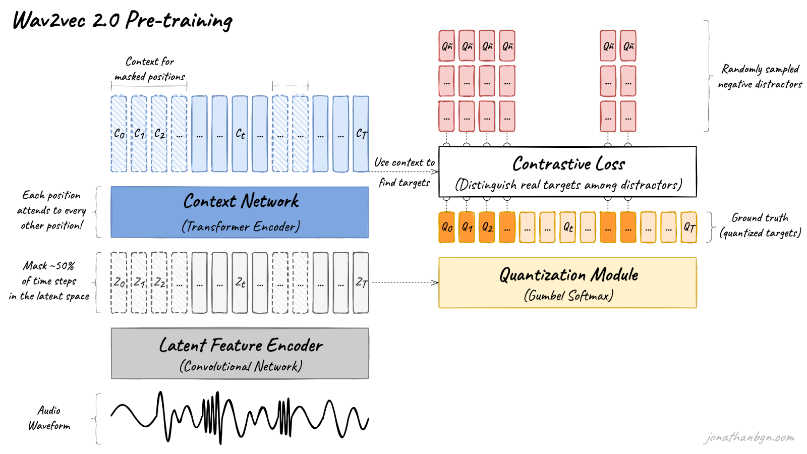
Above is an overview of the wav2vec 2.0 architecture and its pre-training process. There are four important elements in this diagram: the feature encoder, context network, quantization module, and a contrastive loss (pre-training objective). We will open the hood and look in detail at each one.
Feature encoder
The feature encoder’s job is to reduce the dimensionality of the audio data, converting the raw waveform into a sequence of feature vectors Z0, Z1, Z2, …, ZT every 20 milliseconds. Its architecture is simple: a 7-layer convolutional neural network (single-dimensional) with 512 channels at each layer.
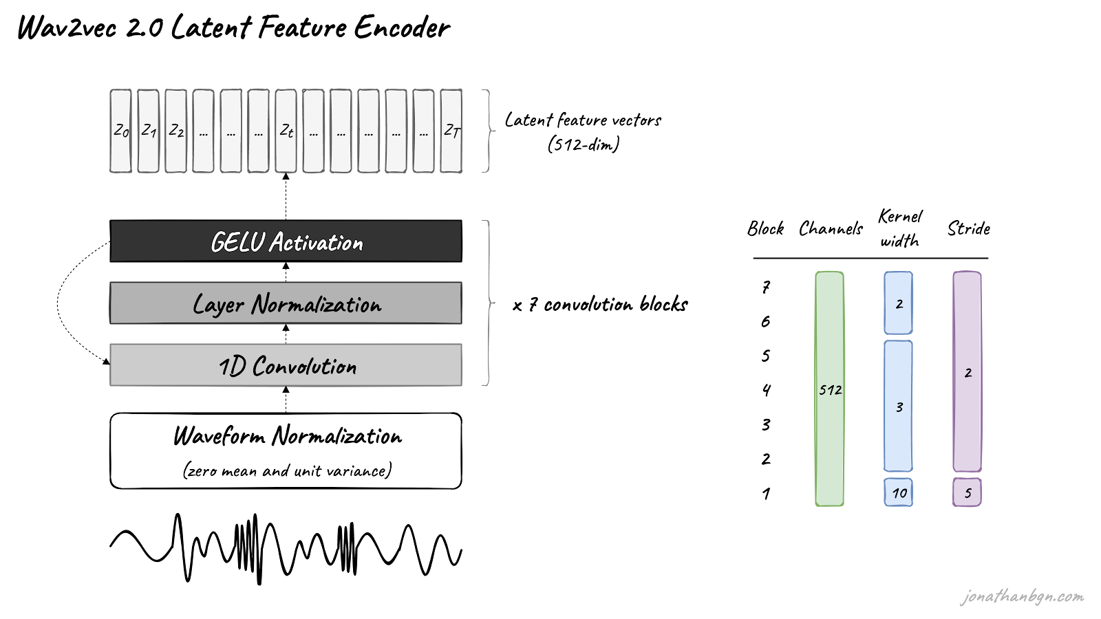
The waveform is normalized before being sent to the network, and the kernel width and strides of the convolutional layers decrease as we get higher in the network. The feature encoder has a total receptive field of 400 samples or 25 ms of audio (audio data is encoded at a sample rate of 16 kHz).
Quantization module
Wav2vec 2.0 proposes to automatically learn discrete speech units, by sampling from a Gumbel-Softmax distribution. Possible units are made of codewords sampled from codebooks (groups). Codewords are then concatenated to form the final speech unit. Wav2vec uses 2 groups with 320 possible words in each group, hence a theoretical maximum of 320 x 320 = 102,400 speech units.
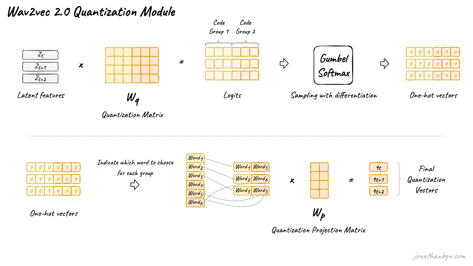
The latent features are multiplied by the quantization matrix to give the logits: one score for each of the possible codewords in each codebook. The Gumbel-Softmax trick allows sampling a single codeword from each codebook, after converting these logits into probabilities. It is similar to taking the argmax, except that the operation is fully differentiable. Moreover, a small randomness effect, whose effect is controlled by a temperature argument, is introduced to the sampling process to facilitate training and codewords utilization.
Context network
The core of wav2vec 2.0 is its Transformer encoder, which takes as input the latent feature vectors and processes it through 12 Transformer blocks for the BASE version of the model, or 24 blocks for the LARGE version. To match the inner dimension of the Transformer encoder, the input sequence first needs to go through a feature projection layer to increase the dimension from 512 (output of the CNN) to 768 for BASE or 1,024 for LARGE. I will not describe further the Transformer architecture here and invite you to read The Illustrated Transformer for the details.
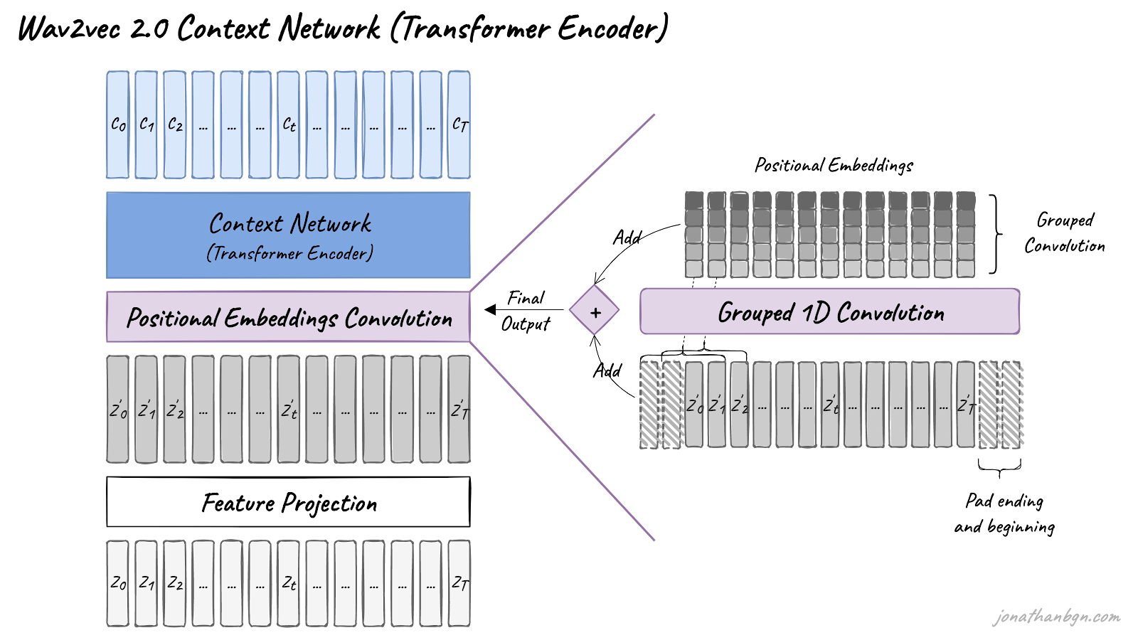
One difference from the original Transformer architecture is how positional information is added to the input. Since the self-attention operation of the Transformer doesn’t preserve the order of the input sequence, fixed pre-generated positional embeddings were added to the input vectors in the original implementation. The wav2vec model instead uses a grouped convolution layer to learn relative positional embeddings by itself.
Pre-training & contrastive loss
The pre-training process uses a contrastive task to train on unlabeled speech data. A mask is first randomly applied in the latent space to ~50% of the projected latent feature vectors. Masked positions are then replaced by the same trained vector Z’M before being fed to the Transformer network.
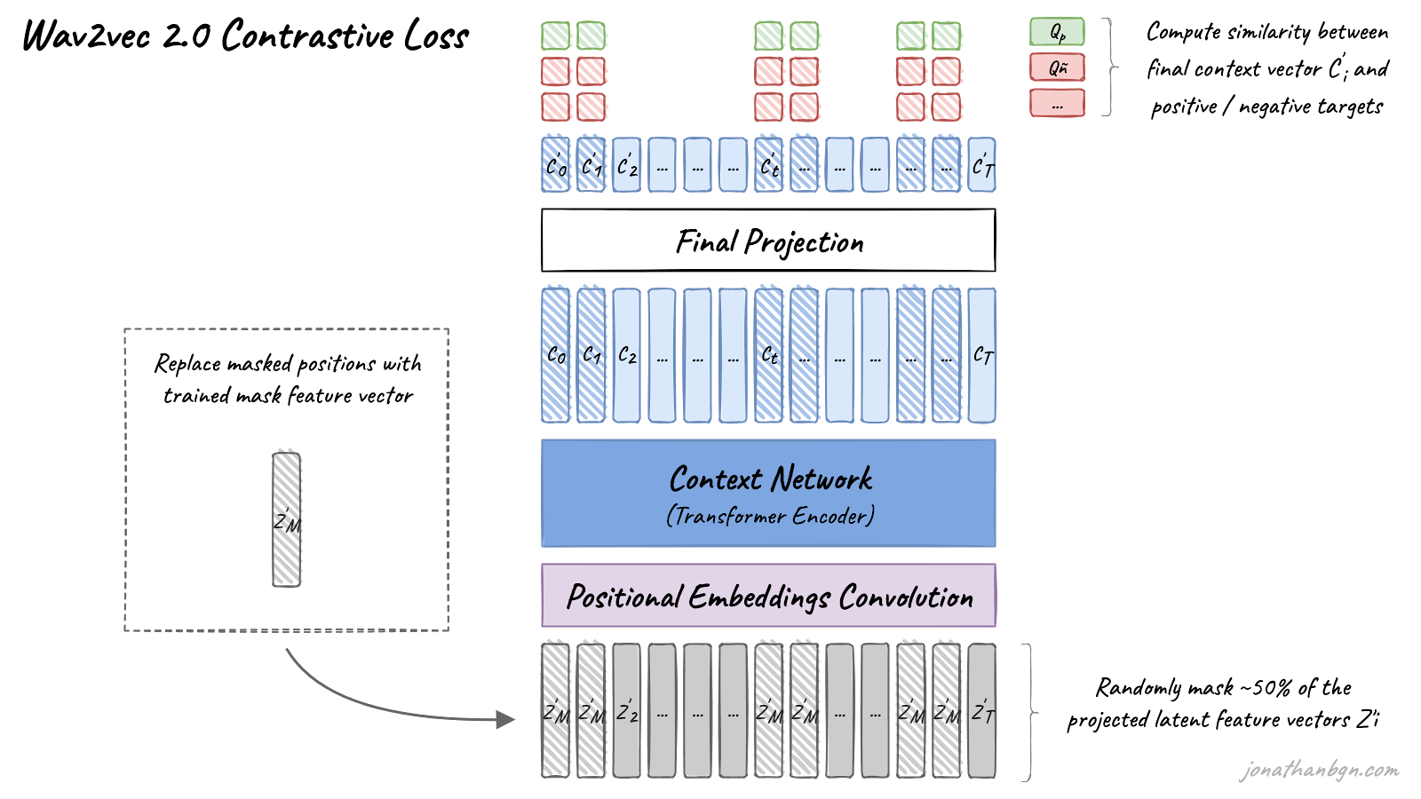
The final context vectors then go through the last projection layer to match the dimension of the quantized speech units Qt. For each masked position, 100 negative distractors are uniformly sampled from other positions in the same sentence. The model then compares the similarity (cosine similarity) between the projected context vector C’t and the true positive target Qp along with all negative distractors Qñ. The contrastive loss then encourages high similarity with the true positive target and penalizes high similarity scores with negative distractors.
Diversity loss
During pre-training, another loss is added to the contrastive loss to encourage the model to use all codewords equally often. This works by maximizing the entropy of the Gumbel-Softmax distribution, preventing the model from always choosing from a small sub-group of all available codebook entries. You can find more details in the original paper.
Fine-tuning and downstream tasks
This concludes our tour of wav2vec 2.0 and its pre-training process. The resulting pre-trained model can then be used for a variety of speech downstream tasks: automatic speech recognition, emotion detection, speaker recognition, language detection, etc. In wav2vec 2.0’s original paper, the authors directly fine-tuned the model for speech recognition with a CTC loss, adding a linear projection on top of the context network to predict a word token at each timestep. They demonstrated that fine-tuning the model this way on only one hour of labeled speech data could beat the previous state-of-the-art systems trained on 100 times more labeled data.
HuBERT
Now let’s look at our second model. HuBERT’s main idea is to discover discrete hidden units (the Hu in the name) to transform speech data into a more “language-like” structure. These hidden units could be compared to words or tokens in a text sentence.
The method draws inspiration from the DeepCluster paper in computer vision, where images are assigned to a given number of clusters before re-using these clusters as “pseudo-labels” for training the model in a self-supervised way. In HuBERT’s case, clustering is not applied on images but on short audio segments (25 milliseconds), and the resulting clusters become the hidden units that the model will be trained to predict.
Differences with wav2vec 2.0
At first glance, HuBERT looks very similar to wav2vec 2.0: both models use the same convolutional network followed by a transformer encoder. However, their training processes are very different, and HuBERT’s performance, when fine-tuned for automatic speech recognition, either matches or improves upon wav2vec 2.0. Here are the key differences to keep in mind:
HuBERT uses the cross-entropy loss, instead of the more complex combination of contrastive loss + diversity loss used by wav2vec 2.0. This makes training easier and more stable since this is the same loss that was used in the original BERT paper.
HuBERT builds targets via a separate clustering process, while wav2vec 2.0 learns its targets simultaneously while training the model (via a quantization process using Gumbel-softmax). While wav2vec 2.0 training could seem simpler as it consists of only a single step, in practice, it can become more complex as the temperature of the Gumbel-softmax must be carefully adjusted during training to prevent the model from “cheating” and sticking to a small subset of all available targets.
HuBERT re-uses embeddings from the BERT encoder to improve targets, while wav2vec 2.0 only uses the output of the convolutional network for quantization. In the HuBERT paper, the authors show that using such embeddings from intermediate layers of the BERT encoder leads to better targets quality than using the CNN output.
In terms of model architecture, the BASE and LARGE versions of HuBERT have the same configuration as the BASE and LARGE versions of wav2vec 2.0 (95 million and 317 million parameters respectively). However, an X-LARGE version of HuBERT is also used with twice as many transformer layers as in the LARGE version, with almost 1 billion parameters.
Training process
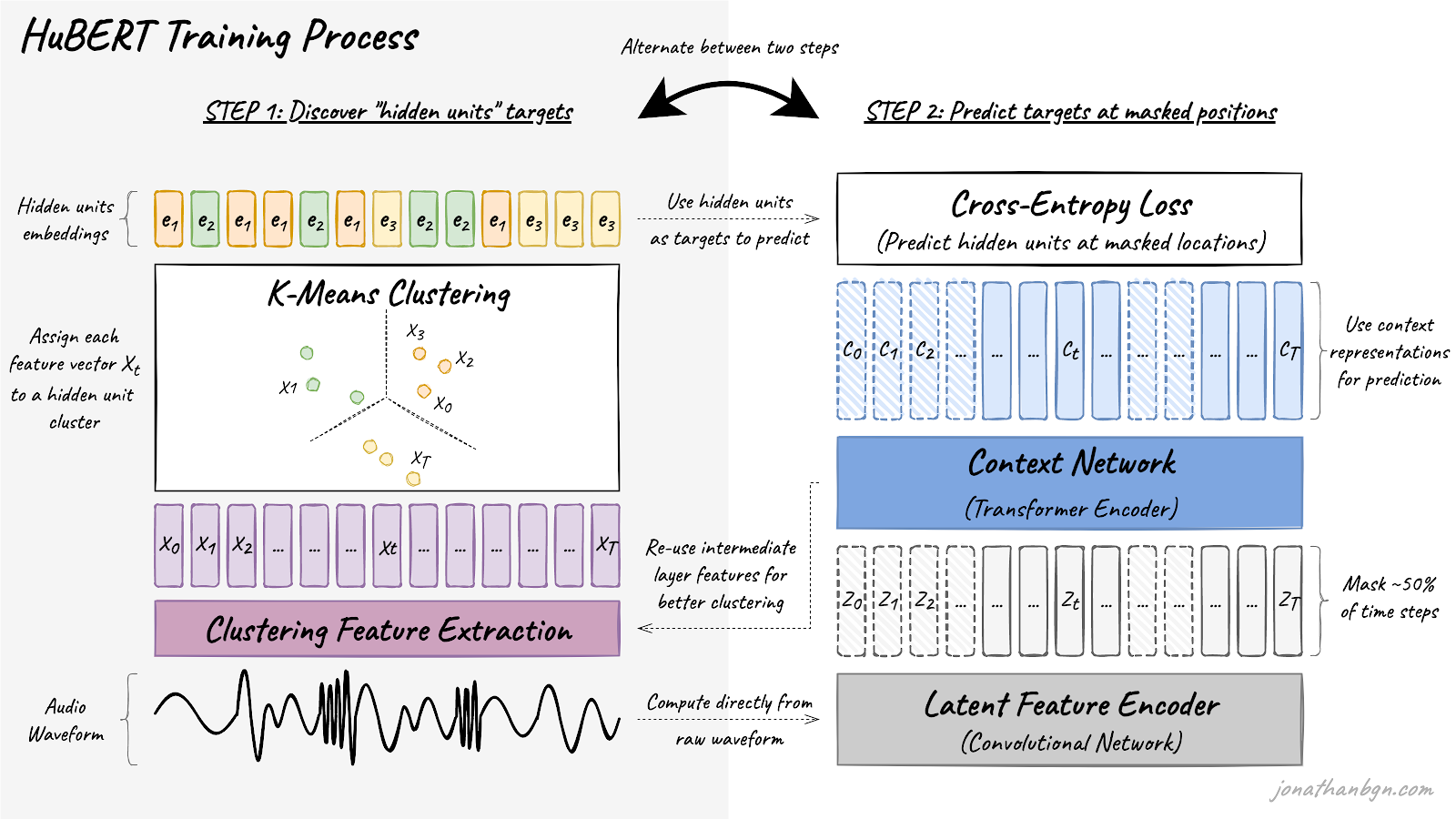
The training process alternates between two steps: a clustering step to create pseudo-targets, and a prediction step where the model tries to guess these targets at masked positions.
Step 1: Discover “hidden units” targets through clustering
The first step is to extract the hidden units (pseudo-targets) from the raw waveform of the audio. The K-means algorithm is used to assign each segment of audio (25 milliseconds) to one of K clusters. Each identified cluster will then become a hidden unit, and all audio frames assigned to this cluster will be assigned with this unit label. Each hidden unit is then mapped to its corresponding embedding vector that can be used during the second step to make predictions.
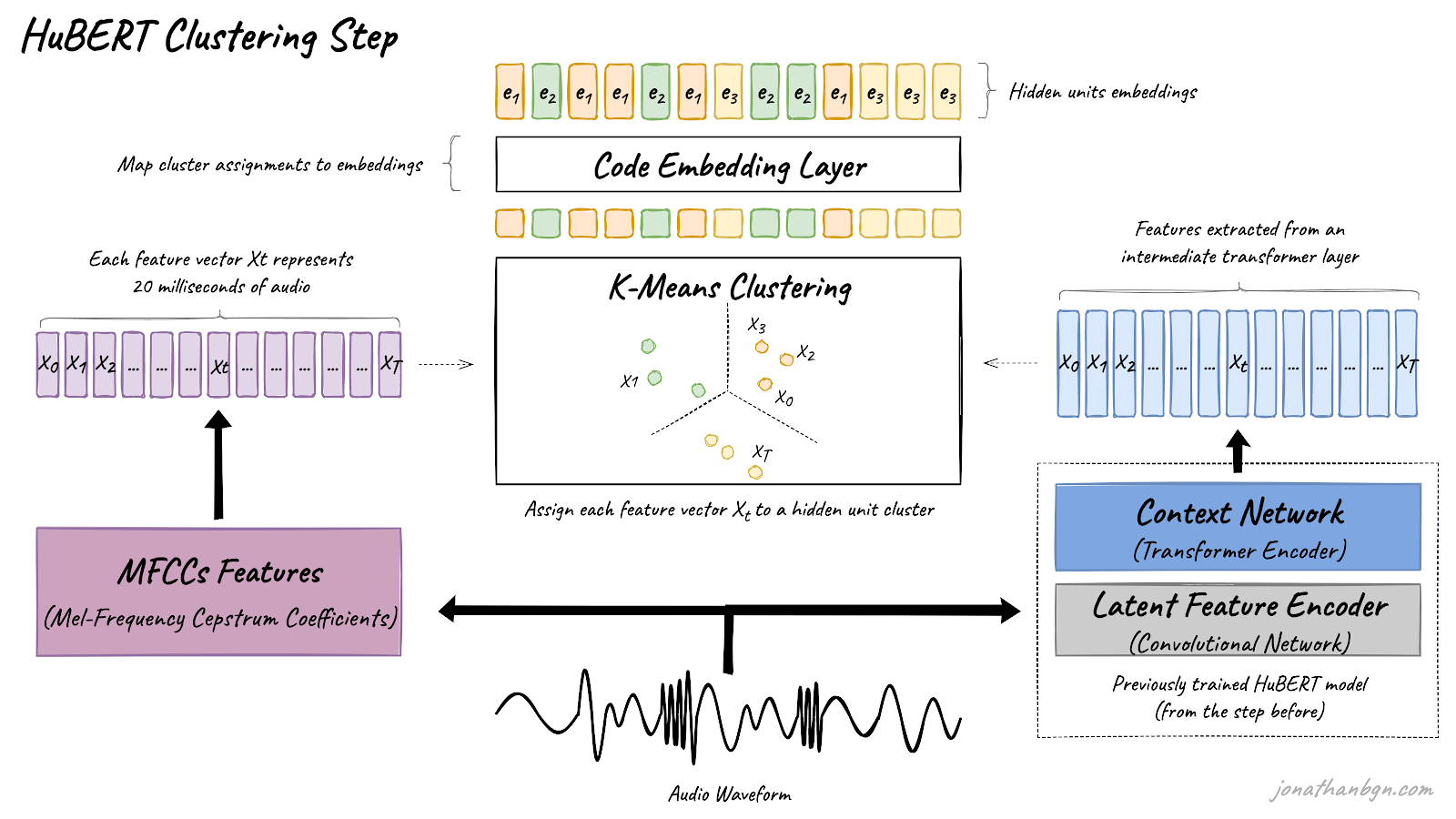
The most important decision for clustering is into which features to transform the waveform for clustering. Mel-Frequency Cepstral Coefficients (MFCCs) are used for the first clustering step, as these features have been shown to be relatively efficient for speech processing. However, for subsequent clustering steps, representations from an intermediate layer of the HuBERT transformer encoder (from the previous iteration) are re-used.
More precisely, the 6th transformer layer is used for clustering during the second iteration of the HuBERT BASE model (the BASE model is only trained for two iterations in total). Furthermore, HuBERT LARGE and X-LARGE are trained for a third iteration by re-using the 9th transformer layer from the second iteration of the BASE model.
Combining clustering of different sizes
The authors also experiment with a combination of multiple clustering with a different number of clusters to capture targets of different granularity ( vowel/consonant vs sub-phone states for example). They show that using cluster ensembles can improve performance by a small margin. You can find more details on this in the original paper.
Step 2: Predict noisy targets from the context
The second step is the same as for the original BERT: training with the masked language modeling objective. Around 50% of transformer encoder input features are masked, and the model is asked to predict the targets for these positions. For this, the cosine similarity is computed between the transformer outputs (projected to a lower dimension) and each hidden unit embedding from all possible hidden units to give prediction logits. The cross-entropy loss is then used to penalize wrong predictions.
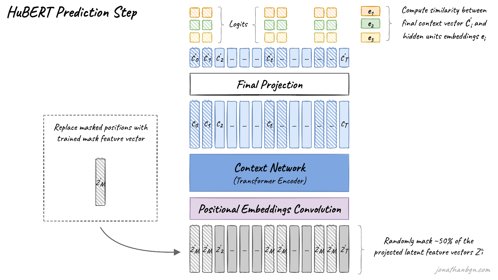
The loss is only applied to the masked positions as it has been shown to perform better when using noisy labels. The authors prove this experimentally by trying to predict only masked targets, only un-masked ones, or both together.
Towards larger, multilingual BERT-like models for speech
Like wav2vec 2.0 before it, HuBERT representations can be reused to improve performance on many downstream tasks such as automatic speech recognition. While these two models are only one part of all BERT-like approaches for speech representation, they offer a great introduction to the current state-of-the-art. Indeed, most of today's large Transformer-based models for speech use similar concepts and ideas.
More generally, the concepts behind both Wav2vec 2.0 and HuBERT open the door to the broader use of NLP algorithms for speech (not just BERT), originally designed only for text sequence. Many of these NLP approaches enable efficient training on unlabeled data.
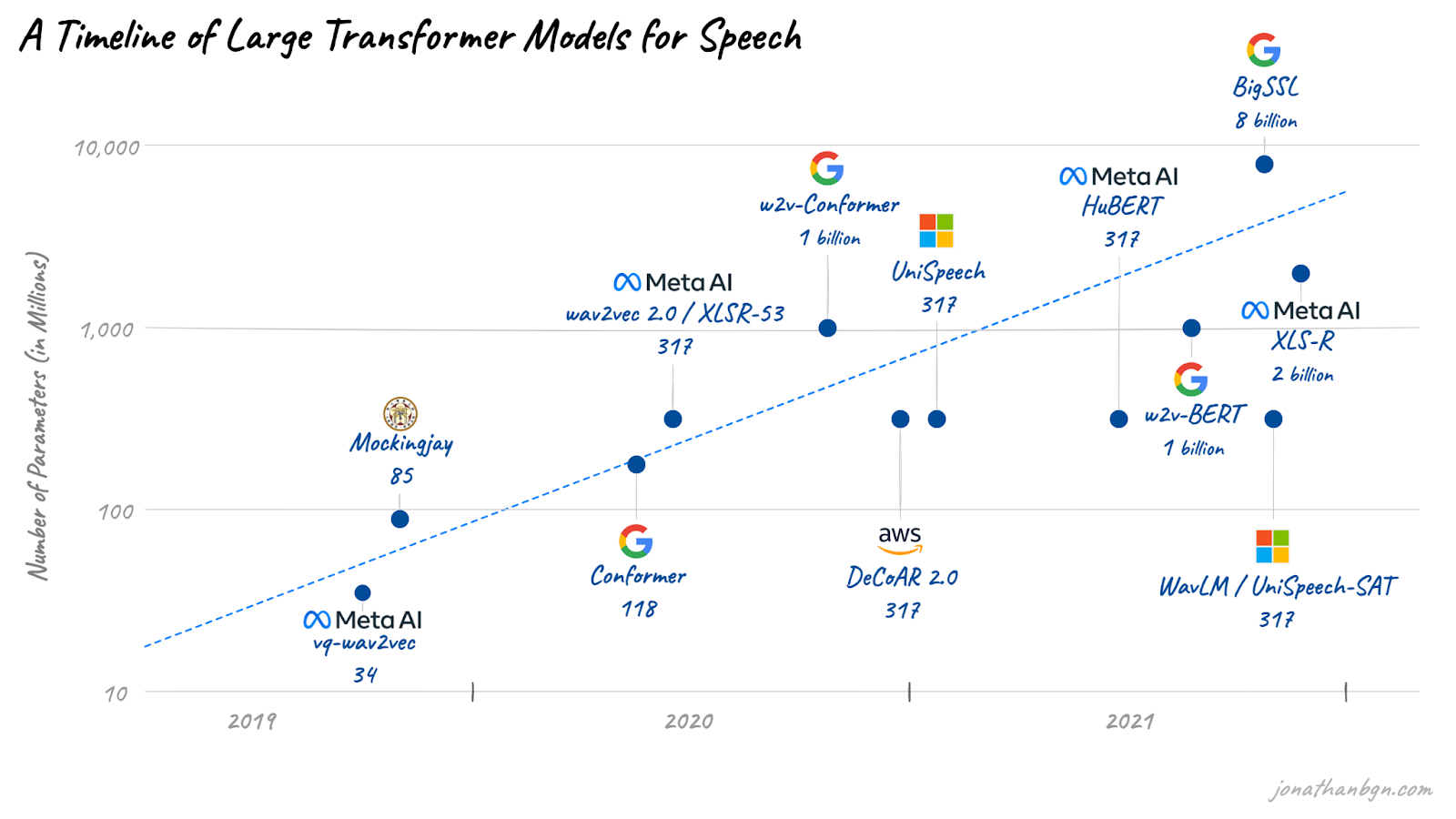
Training on unlabeled acoustic data allows scaling up speech models to very large sizes. While current model sizes are not yet comparable to what we see for text-based models like GPT-3 (175 billion parameters), they are rapidly catching up. More and more large-scale speech datasets are being released, like Common Voice, recorded in diverse languages. These will help train better and more resilient speech models that generalize well in all conditions and environments, a key challenge for speech processing.
Author Bio
Jonathan Boigne is a machine learning engineer specializing in natural language processing and speech, which he regularly writes about on his blog at jonathanbgn.com. His core interests include self-supervised learning, transfer learning, and how to leverage large-scale unlabeled data to improve performance on real-world problems where labels are scarce.

