The message-passing paradigm has been the “battle horse” of deep learning on graphs for several years, making graph neural networks a big success in a wide range of applications, from particle physics to protein design. From a theoretical viewpoint, it established the link to the Weisfeiler-Lehman hierarchy, allowing to analyse the expressive power of GNNs. We argue that the “node and edge-centric” mindset of current graph deep learning schemes imposes strong limitations that hinder future progress in the field. As an alternative, we propose physics-inspired “continuous” learning models that open up a new trove of tools from the fields of differential geometry, algebraic topology, and differential equations so far largely unexplored in graph ML.
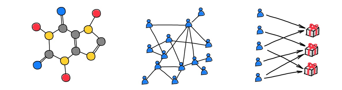
Graphs are a convenient way to abstract complex systems of relations and interactions. The increasing prominence of graph-structured data from social networks to high-energy physics to chemistry, and a series of high-impact successes have made deep learning on graphs one of the hottest topics in machine learning research [1]. Graph Neural Networks (GNNs) are by far the most common among graph ML methods and the most popular neural network architectures overall [2].
How do GNNs work?
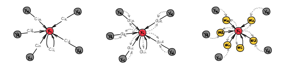
Graph neural networks take as input a graph endowed with node and edge features and compute a function that depends both on the features and the graph structure. Message-passing type GNNs, also called Message Passing Neural Networks (MPNN) [3], propagate node features by exchanging information between adjacent nodes. A typical MPNN architecture has several propagation layers, where each node is updated based on the aggregation of its neighbours’ features. Aggregation functions are typically parametric, and come in three different “flavours” of graph neural networks [4]:
- convolutional: linear combination of neighbour features where weights depend only on the structure of the graph
- attentional: linear combination, where weights are computed based on the features
- message passing: a general nonlinear function dependent on the features of two nodes sharing an edge.
Of these three flavours, the latter is the most general and the two others can be seen as special cases of message passing.
The parameters of propagation layers are learned based on the downstream tasks. Typical use cases include:
- node embedding: representing each node as a point in a vector space in such a way that the proximity of these points recovers the connectivity of the original graph, a task known as “link prediction”
- node-wise classification or regression: for example inferring attributes of social network users
- graph-wise classification or regression: for example, predicting chemical properties of molecular graphs
What’s wrong with message passing GNNs?
It is fair to say that the predominant model underlying current GNNs is message passing. We believe it is this very “node-and-edge-centric” mindset that hinders future progress in the field due to several important limitations:
The Weisfeiler-Lehman analogy is limiting
An appropriate choice of the local aggregation function like summation [5] makes message passing equivalent to the Weisfeiler-Lehman graph isomorphism test [6], allowing graph neural networks to discover some structure of the graph from the way information propagates on it. This important link to graph theory [7] has produced multiple theoretical results on the expressive power of GNNs, determining whether certain functions on a graph can be computed by means of message passing or not [8]. However, these results are not generally informative of the efficiency of such representations (i.e., how many layers are required to compute a function) [9], nor about the generalisation capabilities of GNNs.
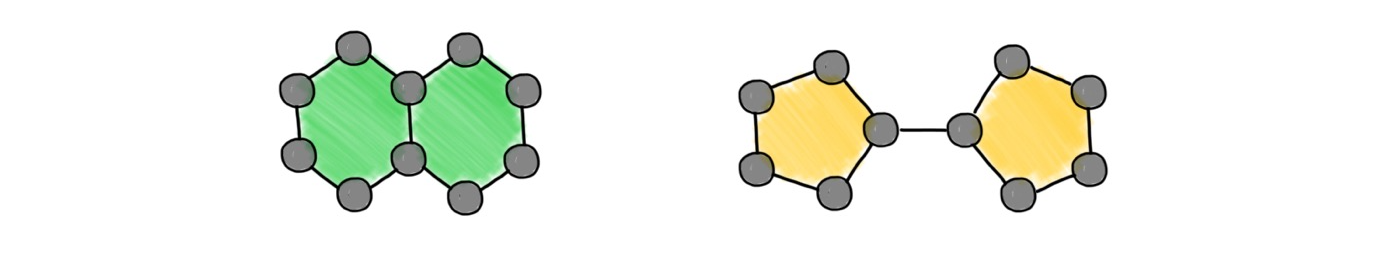
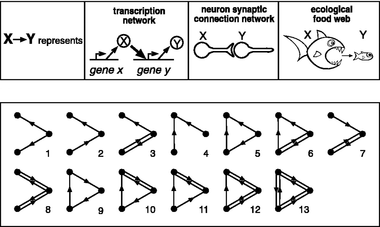
The inability of the Weisfeiler-Lehman algorithm to detect even simple graph structures such as triangles is astonishingly disappointing for practitioners trying to use message passing neural networks for molecular graphs. In organic chemistry, for example, structures such as rings are abundant and play an important role in the way molecules behave.
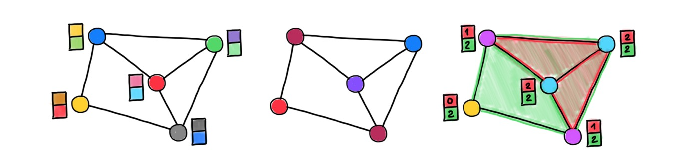
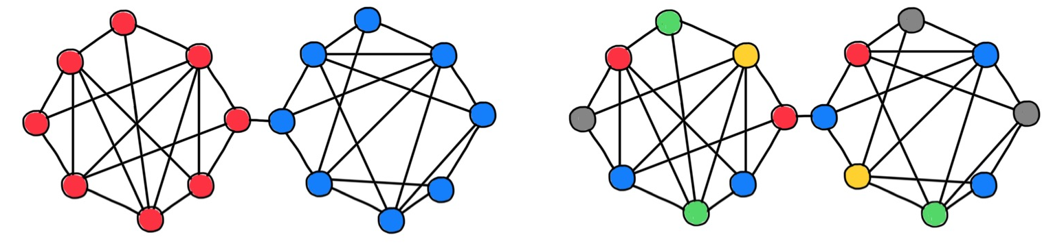
Several approaches have been proposed to improve the expressiveness of GNN models. These include higher-dimensional isomorphism tests in the Weisfeiler-Lehman hierarchy [10]. This approach comes at the expense of higher computational and memory complexity, and lack of locality. Applying the Wesifeiler-Lehman test to a collection of subgraphs [11], or positional- or structural encoding [12] that "colours'' graph nodes to help break the regularities that “confuse” the Weisfeiler-Lehman algorithm. Positional encoding is by far the most common technique borrowed from Transformers [13], it is now ubiquitous in GNNs. While multiple positional encodings exist, it is fair to say that a particular choice is application-dependent and rather empirical.
Graph rewiring breaks the theoretical foundations of GNNs
One important and somewhat subtle difference between GNNs and Convolutional Neural Networks (CNNs) is that the graph is both part of the input and the computational structure. Traditional GNNs use the input graph to propagate information, thus obtaining a representation that reflects both the structure of the graph and its features. However, some graphs turn out to be less “friendly” for information propagation due to certain structural characteristics. These characteristics are called “bottlenecks”, and result in information from too many nodes to be “squeezed” into a single node representation – a phenomenon referred to as “oversquashing” [14].
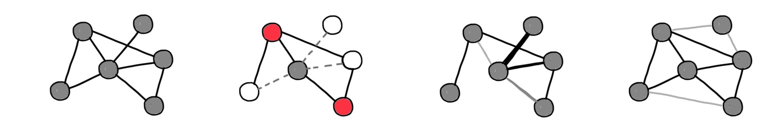
Modern GNN implementations cope with this phenomenon by decoupling the input graph from the computational one (or refining it for computational purposes), a technique known as “graph rewiring”. Rewiring can take the form of neighbourhood sampling (as done in GraphSAGE [15], originally to deal with scalability), virtual nodes [16], connectivity diffusion [17] or evolution [18], or node- and edge-dropout mechanisms [19]. Transformers and attention-type GNNs such as GAT [20] effectively “learn” a new graph by assigning a different weight to each edge, which can also be understood as a form of “soft” rewiring. Finally, “latent graph learning” methods build a task-specific graph and update it at every layer [21], starting with some positional encoding, initial graph, or sometimes with no graph at all. Overall, almost no modern GNN model propagates information on the original input graph.
This is bad news for theoretical analyses relying on the equivalence of message passing and the Weisfeiler-Lehman test to obtain a description of the graph from the way information propagates on it. Rewiring breaks this theoretical link, creating a situation not uncommon in machine learning: models that can be analysed in theory are not the same as those used in practice.
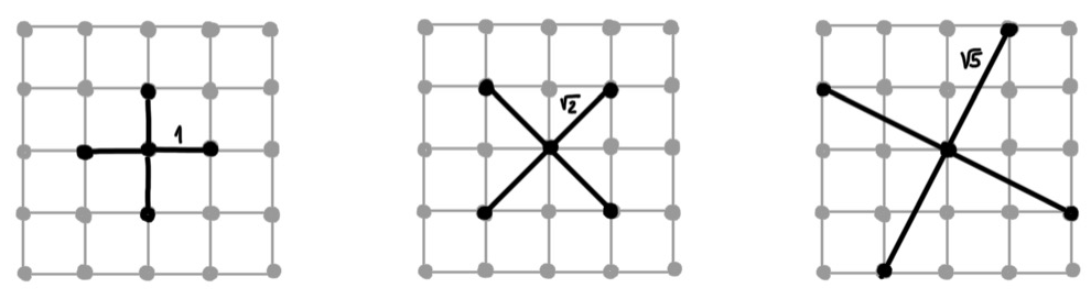
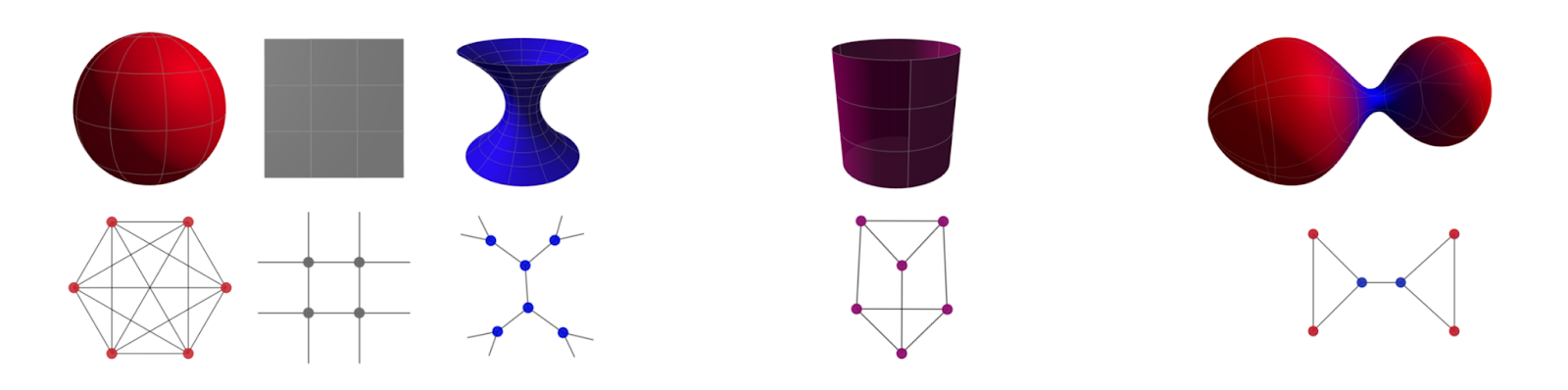
The “geometry” of graphs is too poor
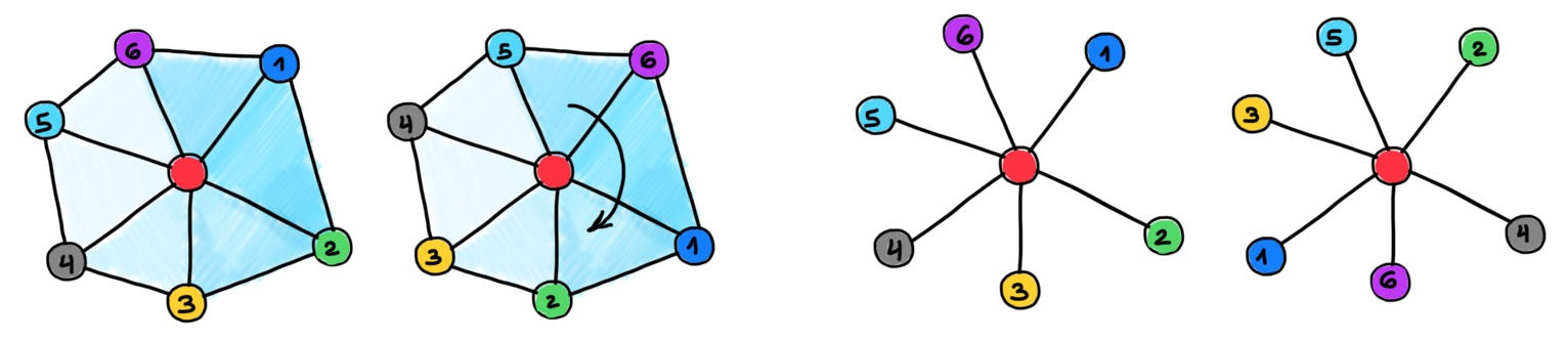
Graph neural networks can be obtained as an instance of the "Geometric Deep Learning blueprint" [22], a group-theoretical framework allowing to derive deep learning architectures from the symmetry of the domain underlying the data. In graphs, this symmetry is node permutation, as graphs do not have a canonical node ordering. Because of this structural characteristic, MPNNs operating locally on the graph must rely on permutation-invariant feature aggregation functions. This implies that graphs have no straightforward notion of "direction", and that the propagation of information is isotropic [23]. This situation is strikingly different from learning on continuous domains, grids, or even meshes [24], and has been one of the early criticisms of GNNs arguing that isotropic filters are not very useful [25].
The “geometry” of graphs is too rich
On the other hand, graphs might have structures that are not compatible with standard spaces used for their representations. When building node embeddings, the distance between the vector representations of the nodes is used to capture the connectivity of the graph. In short, nodes close in the embedding space are expected to be connected by an edge in the graph. Typical use cases are recommender systems, where graph embeddings are used to create associations (edges) between entities represented by the nodes (e.g., whom to follow on Twitter).
The quality of graph embeddings and their ability to convey the structure of the graph crucially depends on the geometry of the embedding space and its compatibility with the "geometry" of the graph. Euclidean spaces, a staple of representation learning and by far the simplest and most convenient to work with, can be a poor choice for many natural graphs. One of the reasons is that the volume growth of Euclidean metric balls is polynomial in the radius but exponential in the dimension [26]. In contrast, many real-world graphs manifest exponential volume growth [27]. As a result, embeddings become "too crowded", forcing the use of high dimensional embedding spaces that come with higher computational and space complexity.
A recently popular alternative is to use hyperbolic (negatively-curved) spaces [28] that have exponential volume growth more compatible with that of graphs [29]. The use of hyperbolic geometry typically leads to lower embedding dimensions, resulting in more compact node representations. However, this is not enough: graphs often tend to be heterogeneous, and some parts may look like trees and others as cliques, with very different volume growth properties. On the other hand, hyperbolic and Euclidean embedding spaces are homogeneous, meaning that every point has the same geometry.
Furthermore, it is generally impossible to exactly represent the metric structure of a general graph in an embedding space [30], even using non-Euclidean geometry. Thus, graph embeddings are inevitably approximate. Moreover, since embeddings are constructed with "link prediction" in mind, the distortion of higher-order structures (triangles, rectangles, etc.) can be uncontrollably large [31]. In some applications, including social and biological networks, such structures play an important role as they capture complex non-pairwise interactions and motifs [32].
GNNs struggle when data structure is not compatible with the underlying graph structure
Many graph learning datasets and benchmarks make the tacit assumption that the features or labels of adjacent nodes are similar, a property called homophily. In this setting, even simple low-pass filtering on the graph (e.g., taking the neighbour average) tends to work well. Early benchmarks, including the still ubiquitous Cora dataset, were graphs with a high level of homophily. Many models however show disappointing results when dealing with heterophilic data, where more nuanced aggregation is required [33]. Typically the model then either ignores neighbour information altogether, or node representations become smoother with every layer of GNN, eventually collapsing into a single point [34]. The latter phenomenon also occurs in homophilic datasets and appears to be a more fundamental plight of some types of MPNNs, making it hard to implement deep graph learning models [35].
GNNs are hard to interpret
Several recent works try to mitigate this issue by providing interpretation methods for GNN-based models. These can take the form of compact subgraph structures, or a small subset of node features that have a crucial role in GNN's prediction [36]. Restricting generic message-passing functions helps ruling out implausible outputs and ensures that what the GNN learns suits domain-specific applications. In particular, it is possible to endow message passing with additional “internal” data symmetries that better fit the underlying problem [37]. A perfect example is E(3)-equivariant message passing that correctly treats the atomic coordinates in molecular graphs and has recently contributed to the breakthroughs in protein structure prediction with architectures such as AlphaFold [38] and RosettaFold [39].
Another example is the work coauthored by Miles and Kyle Cranmer (no family relation) [40]. In this work, message-passing functions learned on a multi-body dynamical system were replaced by symbolic formulae. Allowing the model to learn physical equations. Finally, attempts were made to link GNNs to causal inference [41]. Here one tries to build a graph explaining the causal relations between different variables. Overall, this is still a research domain in its infancy, and much remains to be discovered.
Lack of GNN specific hardware
The majority of today's GNNs rely on GPU implementation and tacitly assume that the data fits into memory. This assumption is often wrong when dealing with large graphs such as biological and social networks. In these cases, understanding the limitations of the underlying hardware such as different bandwidth and latency of the memory hierarchy is of crucial importance.. There might be an order of magnitude difference in the cost of message passing (in terms of latency and power, for example) between two nodes in the same physical memory and two nodes on different chips. Making GNNs friendly to existing hardware is an important and frequently overlooked problem. Developing novel graph-centric hardware is an even bigger challenge, given the time and effort it takes to design a new chip, and the speed at which machine learning state-of-the-art moves.
Reimagining GNNs as continuous physical processes
An emerging and promising alternative to current GNN paradigms are continuous learning models that are inspired by physical systems and open up a new trove of tools from the fields of differential geometry, algebraic topology, and differential equations so far largely unexplored in graph ML.
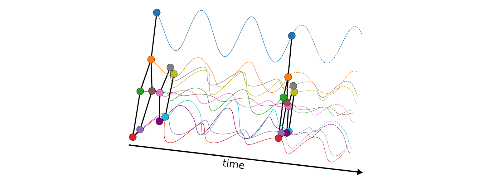
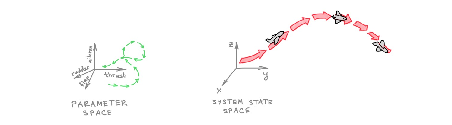
Instead of several layers of message passing on a graph, we consider a continuous-time physical process on some domain. This domain can be a continuous manifold discretised as a graph. The state of the process at given points in space and time replace the latent features of nodes of the graph produced by the layers of GNNs. The process is controlled by a set of parameters, representing the properties of the underlying physical system. These parameters replace the learnable weights of message passing layers.
A plethora of different physically-inspired processes can be drawn from both classical and quantum systems. In a series of papers [42–44], we have shown that many existing GNNs can be related to diffusion processes, which are probably the most natural way of propagating information, but other more exotic ways, such as systems of coupled oscillators [45] are also possible and may offer certain advantages.
A continuous system can be discretised both in time and space. The spatial discretisation takes the form of a graph connecting nearby points on the continuous domain, and can change throughout both time and space. Such a learning paradigm is a radical departure from the traditional Weisfeiler-Lehman scheme that is rigidly bound by the assumption of the underlying input graph. More importantly, it brings a new set of tools allowing, at least in principle, to address important questions that are presently out of reach of the existing graph-theoretical frameworks.
Learning as an optimal control problem
The space of all possible states of a process at a given time can be regarded as a hypothesis class of functions to be represented. Framed this way, learning is posed as an optimal control problem [46]. The goal becomes to control the process, by choosing a trajectory in the parameter space, to reach a certain desirable state. Using optimal control terminology, expressive power can be formulated as how well a given function can be reached by a trajectory in the parameter space. Efficiency is related to how long it takes to reach a certain state. Finally, generalisation is related to the stability of this process.
GNNs can be derived from discretised differential equations
The behaviour of physical systems is typically governed by differential equations whose solutions produce the state of the system. In some cases, such solutions can be derived in a closed form [47], but more generally, one has to resort to numerical solutions based on appropriate discretisations. The wealth of different iterative solvers accumulated in the numerical analysis literature after over a century of research offers potentially completely new architectures for deep learning on graphs.
For example, we showed in [42] that attentional flavours of GNNs can be interpreted as discretised diffusion PDEs with learnable diffusivity solved using explicit numerical schemes. In this case, each iteration of the solver (discrete steps in time) corresponds to a layer of a GNN. More sophisticated solvers, like using adaptive step size or multi-step schemes do not currently have an immediate analogy with current GNN architectures, and could lead to future architectural insights. Implicit schemes, requiring the solution of a linear system at each iteration, can be interpreted as “multi-hop” filters [48]. Furthermore, numerical schemes come with stability and convergence guarantees, providing conditions when they work and an understanding when they fail [49].
Numerical solvers can be hardware-friendly
Iterative solvers are older than computers, and from the very beginning of the digital computers era, the former had to be aware of the latter. Large-scale problems in scientific computing often have to be solved on clusters of computers, where such issues are of crucial importance.
The continuous approach to deep learning on graphs allows discretising the underlying differential equations in ways that are compatible with the hardware on which they are simulated, potentially leveraging vast literature from the supercomputing community such as domain decomposition techniques [50]. In particular, graph rewiring and adaptive iterative solvers can be made aware of memory hierarchy. They can, for example, perform fewer infrequent steps of information transfer across nodes in different physical locations and more frequent steps across nodes in the same physical memory.
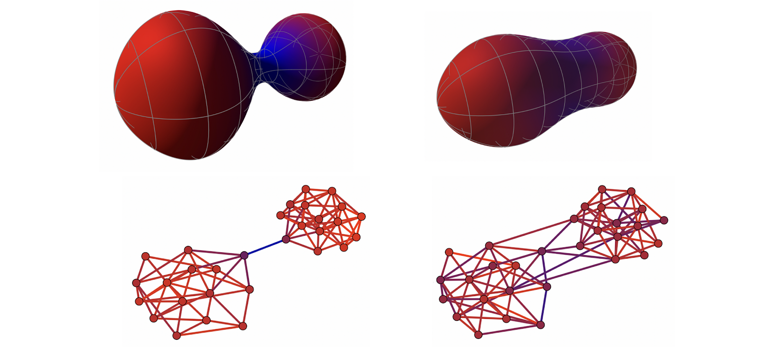
Interpreting evolution equations as gradient flows of energy functionals associated with a physical system provides insights into the learning model. Many physical systems have an associated energy functional, of which the differential equation governing the dynamics of the system is a minimising gradient flow [51]. For example, the diffusion equation minimises the Dirichlet energy [42] and its non-Euclidean version (Beltrami flow) minimises the Polyakov functional [43], giving an intuitive grasp on what the learning model is doing. Using the principle of least action w.r.t. certain energy functionals lead to hyperbolic equations, such as the wave equation. The solutions of such equations are “wave-like” (oscillatory) and dramatically different from the typical dynamics of GNNs.
Analysing the limit cases of such flows is a standard exercise that provides deep insight on the behaviour of the model that would be difficult to gain otherwise. For example, in our recent paper [44] we showed that traditional GNNs (analogous to isotropic diffusion equations) necessarily lead to oversmoothing and have separation power only under the assumption of homophily; better separation power can be achieved by using additional structure on the graph (a cellular sheaf) [52]. In another recent paper [45], we showed that an oscillatory system avoids oversmoothing in the limit. Such results can explain why certain undesirable phenomena occur in some GNN architectures, and how to design architectures to avoid them. Furthermore, linking the limit case of the flow to separation reveals bounds on the expressive power of the model.
Graphs can be endowed with richer structures
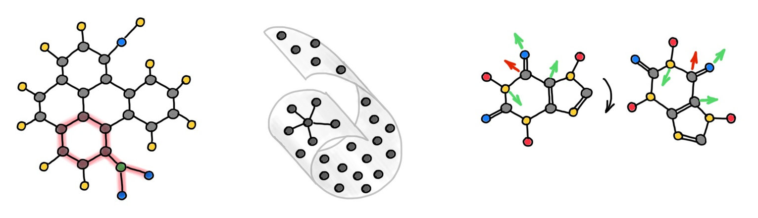
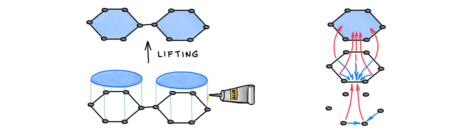
We already mentioned that graphs may be “too poor” (i.e., fail to capture more complex phenomena like non-pairwise relations) and “too rich” (i.e., hard to be represented in a homogeneous space) at the same time. A way to deal with the former problem is to “enrich” the graph with additional structures. A good example is molecular graphs containing rings (cycles in graph terminology) that chemists regard as single entities rather than just a collection of atoms and bonds (nodes and edges).
In a series of works [53–54] we showed that graphs can be "lifted" to higher-dimensional topological structures called simplicial- and cellular complexes, on which one can design a more complex message passing scheme allowing to propagate information not only between nodes like in traditional GNNs, but also between structures like rings ("cells"). Appropriate construction of the lifting operation makes such models more expressive than the traditional Weisfeiler-Lehman test [55].
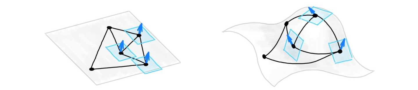
In another recent paper [44], we showed that graphs can be equipped with an additional "geometric" structure called a cellular sheaf by assigning vector spaces and linear maps to nodes and edges. Traditional GNNs implicitly assume a graph with a trivial underlying sheaf, which is reflected in the properties of the associated diffusion equation and the structure of the graph Laplacian operator. Making the sheaf non-trivial (and learnable from the data) produces richer diffusion processes and gives greater control over their asymptotic behaviour compared to traditional GNNs. For example, diffusion equations on an appropriately selected sheaf structure can separate in the limit multiple classes even in heterophilic settings [52].
From the geometric standpoint, the sheaf structure is analogous to a connection, a notion from differential geometry describing the parallel transport of vectors on manifolds [56]. In this sense, one can regard sheaf learning as a way of evolving the "geometric" structure of the graph depending on the downstream task. We show that interesting insights can be gained by restricting the structure group of the sheaf. Using the jargon of algebraic topology, restriction maps can be applied to the special orthogonal group, allowing the node feature vectors to rotate only.
Another example of geometric structures on graphs are discrete analogues of curvature. A standard tool from the field of differential geometry to describe the local behaviour of manifolds. In [18], we showed that negative graph Ricci curvature produces information flow bottlenecks on the graph and resulting in the oversquashing phenomenon in GNNs [14]. Discrete Ricci curvature accounts for higher-order structures (triangles and rectangles) that are important in many applications. Such structures are "too rich" for traditional graph embeddings, since graphs are heterogeneous (have non-constant curvature), whereas the spaces commonly used for embeddings, even non-Euclidean ones, are homogeneous (constant curvature).
In another recent paper [57], we showed a construction of heterogeneous embedding spaces with controllable Ricci curvature that can be chosen to match that of the graph, allowing to better represent not only the neighbourhood (distance) structure but also the higher-order structures such as triangles and rectangles. Such spaces are constructed as products of homogeneous and rotationally-symmetric manifolds and allow for efficient optimisation using standard Riemannian gradient descent methods [58].
Positional encoding can be regarded as part of the domain
Thinking of a graph as a discretisation of a continuous manifold, one can consider the node positional and feature coordinates as different dimensions of the same space. The graph in this case can be used to represent a discrete analogue of a Riemannian metric induced by such an embedding. The harmonic energy associated with the embedding is a non-Euclidean extension of the Dirichlet energy, known as the Polyakov functional in string theory [59]. The gradient flow of this energy is a diffusion-type equation that evolves both the positional and feature coordinates [43]. Building a graph upon the positions of the nodes is a form of task-specific graph rewiring that changes across the iterations (layers) of the diffusion.
Evolution of the domain replaces graph rewiring
Diffusion equations can also be applied to the connectivity of the graph as a pre-processing step aimed at improving information flow and avoiding oversquashing. Klicpera et al. [17] proposed one such algorithm based on personalised page rank, a form of graph diffusion embedding. In [18], we analysed this process pointing to its problematic behaviour in heterogeneous settings and proposed an alternative graph rewiring scheme by a process inspired by the Ricci flow. Such a rewiring reduces the effect of negatively-curved edges responsible for graph bottlenecks. Ricci flows are geometric evolution equations for manifolds very roughly resembling the diffusion equations applied to the Riemannian metric, and are a popular and powerful technique in differential geometry, including the celebrated proof of the Poincaré conjecture. More generally, instead of performing graph rewiring as a pre-processing step, one can consider a coupled system of evolution processes: one evolving the features and another one evolving the domain (graph).
Concluding remarks
Is this really new? One of the traps we must avoid falling into is basing new models on fancy mathematical formalism, with the underlying models still doing roughly what the previous generation of GNNs did. For example, one can argue that sheaf diffusion studied in [44] is a special case of message passing. The insightful theoretical results that were made possible with tools from differential geometry [18,43] and algebraic topology [44,53–54] suggest that it is unlikely. However, how far can the new theoretical framework take us, and whether it will be able to address the currently unanswered questions in the field is still an open question.
Will these methods be actually used in practice? For practitioners, a crucial question would be whether these methods will result in better architectures, or remain a theoretical apparatus detached from real-world applications used solely to prove theorems. We believe that theoretical insights obtained with topological and geometric tools would allow for better decision making regarding architectural choices and innovation. Our framework could help answer central questions about how and when to restrict message passing functions.
Have we moved beyond message passing? Finally, a question of a somewhat semantic nature is whether the described approaches can still be labelled as "message passing". Opinions vary from casting every form of GNN as message passing [60] to proclaiming the need to go beyond this paradigm [61]. Sensu amplo, any computation on a digital computer is a form of message passing. However, in the sensus strictus of GNNs, message passing is a computational concept implemented by sending information from one node to another, an inherently discrete process.In contrast, the described physical models share information between nodes in a continuous manner. For example, in a system of graph-coupled oscillators, the dynamics of one node depends on that of its neighbours at every point in time. When the differential equations describing such systems are discretised and solved numerically, the corresponding iterative schemes are indeed implemented through message passing.
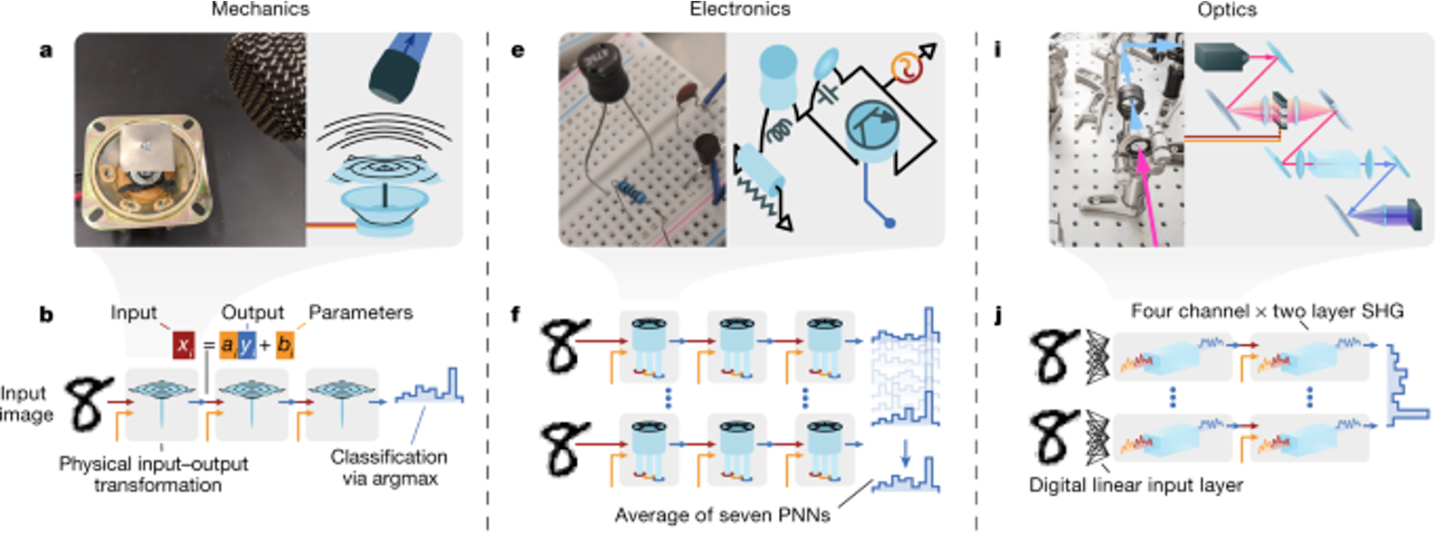
However, one can hypothetically use other physical systems [62] or computing paradigms such as analogue electronics or photonics [63]. Mathematically, the solution of the underlying differential equations may sometimes be given in a closed form: for example, the solution of the isotropic diffusion equation is a convolution with a Gaussian kernel. In this case, the influence of the “neighbours” is absorbed within the structure of the kernel and no actual “message passing” happens. Therefore, the continuous nature of this model calls for a more appropriate term, such as "spatial coupling" or "information propagation" in the absence of better ideas at this time. Nonetheless,, message passing, as computational primitive, is and will likely remain useful, when applied synergistically with additional paradigms such as those presented here.
Acknowledgments
I am grateful to Dominique Beaini, Cristian Bodnar, Giorgos Bouritsas, Ben Chamberlain, Xiaowen Dong, Francesco Di Giovanni, Nils Hammerla, Haggai Maron, Sid Mishra, Christopher Morris, James Rowbottom, and Petar Veličković for very fruitful discussions and comments, some of which were so substantial that amounted to “collective editing”.
This article was edited by Tariq Daouda.
Author Bio
Michael Bronstein is the DeepMind Professor of AI at the University of Oxford and Head of Graph Learning Research at Twitter. He was previously a professor at Imperial College London and held visiting appointments at Stanford, MIT, and Harvard, and has also been affiliated with three Institutes for Advanced Study (at TUM as a Rudolf Diesel Fellow (2017-2019), at Harvard as a Radcliffe fellow (2017-2018), and at Princeton as a short-time scholar (2020)). Michael received his PhD from the Technion in 2007. He is the recipient of the Royal Society Wolfson Research Merit Award, Royal Academy of Engineering Silver Medal, five ERC grants, two Google Faculty Research Awards, and two Amazon AWS ML Research Awards. He is a Member of the Academia Europaea, Fellow of IEEE, IAPR, BCS, and ELLIS, ACM Distinguished Speaker, and World Economic Forum Young Scientist. In addition to his academic career, Michael is a serial entrepreneur and founder of multiple startup companies, including Novafora, Invision (acquired by Intel in 2012), Videocites, and Fabula AI (acquired by Twitter in 2019).
Citation
For attribution in academic contexts or books, please cite this work as
Michael Bronstein, "Beyond Message Passing, a Physics-Inspired Paradigm for Graph Neural Networks", The Gradient, 2022.
BibTeX citation:
@article{michaelbeyond2022,
author = {Bronstein, Michael},
title = {Beyond Message Passing: a Physics-Inspired Paradigm for Graph Neural Networks},
journal = {The Gradient},
year = {2022},
howpublished = {\url{https://thegradient.pub/graph-neural-networks-beyond-message-passing-and-weisfeiler-lehman}},
}
Footnotes
[1] See e.g. ICLR 2021 statistics.
[2] I am counting Transformers as an instance of GNNs.
[3] I use the term “GNN” to refer to an arbitrary graph neural network architecture and “MPNN” for architectures based on local message passing.
[4] Typical representatives of the convolutional flavour are “spectral” graph neural networks that emerged from the domain of graph signal processing such as M. Defferrard et al. Convolutional neural networks on graphs with fast localized spectral filtering (2016) NIPS and T. Kipf and M. Welling, Semi-supervised classification with graph convolutional networks (2017) ICLR. The attentional flavour was introduced by Petar Veličković in [16], though one can consider the Monet architecture developed by F. Monti et al., Geometric deep learning on graphs and manifolds using mixture model CNNs (2017) CVPR, as a form of attention on positional coordinates. A general form of message passing and the name MPNN were used by J. Gilmer et al., Neural message passing for quantum chemistry (2017) ICML.
The naming of the flavours, which we adopted in our “proto-book” M. M. Bronstein et al., Geometric Deep Learning: Grids, Groups, Graphs, Geodesics, and Gauges (2021) arXiv:2104.13478, is due to Petar Veličković. In my earlier versions of this dichotomy (such as the tutorial at MLSS Moscow 2019) I used the terms “linear” (where the feature computation has the form Y=AX with A typically being some form of the graph adjacency matrix), “linear feature dependent” (Y=A(X)X) and “nonlinear” (Y=𝒜(X)). This is less general than the notation adopted in the book, as it assumes sum-based aggregation.
[5] The local aggregation function must be injective. See K. Xu et al. How powerful are graph neural networks? (2019) ICLR.
[6] B. Weisfeiler and A. Lehman, The reduction of a graph to canonical form and the algebra which appears therein (1968). Nauchno-Technicheskaya Informatsia 2(9):12–16.
[7] See C. Morris et al., Weisfeiler and Leman go Machine Learning: The Story so far (2021) arXiv:2112.09992 for historic notes and an in-depth review.
[8] Z. Chen et al., On the equivalence between graph isomorphism testing and function approximation with GNNs (2019) NeurIPS, showed the equivalence between graph isomorphism testing and the approximation of permutation-invariant graph functions.
[9] For example, N. Dehmamy, A.-L. Barabási, R. Yu, Understanding the representation power of graph neural networks in learning graph topology (2019) NeurIPS shows that learning certain functions on graphs (graph moments of certain order) requires GNNs of certain minimum depth. See also F. Geerts and J. L. Reutter, Expressiveness and Approximation Properties of Graph Neural Networks (2022) ICLR.
[10] The hierarchy of so-called “k-WL tests” of strictly increasing power. László Babai credits the invention of the k-WL tests to himself with Rudolf Mathon and independently, Neil Immerman and Eric Lander. See L. Babai, Graph isomorphism in quasipolynomial time (2015), arXiv:1512.03547 p. 27.
[11] There have been several papers proposing to apply GNNs on a collection of subgraphs, including our own B. Bevilacqua et al., Equivariant Subgraph Aggregation Networks (2021) arXiv:2110.02910. See our post on this topic.
[12] Structural encoding by counting local substructures was proposed in the context of GNNs by G. Bouritsas, F. Frasca et al. Improving graph neural network expressivity via subgraph isomorphism counting (2020). arXiv:2006.09252. See also P. Barceló et al., Graph Neural Networks with Local Graph Parameters (2021) arXiv:2106.06707.
[13] A. Vaswani et al., Attention is all you need (2017) NIPS.
[14] The oversquashing phenomenon is not unique to GNNs and has been previously observed also in seq2seq models. However, it can become particularly acute in graphs with exponential volume growth. See U. Alon and E. Yahav, On the bottleneck of graph neural networks and its practical implications (2020). arXiv:2006.05205 and our paper [14] for the description and analysis of this phenomenon.
[15] W. Hamilton et al., Inductive representation learning on large graphs (2017) NIPS used neighbourhood sampling to cope with scalability.
[16] P. W. Battaglia et al., Relational inductive biases, deep learning, and graph networks (2018), arXiv:1806.01261.
[17] J. Klicpera et al., Diffusion improves graph learning (2019) NeurIPS used rewiring through personalised page rank embedding (a form of “connectivity diffusion”).
[18] J. Topping, F. Di Giovanni et al., Understanding over-squashing and bottlenecks on graphs via curvature (2022) ICLR.
[19] Dropout can be done on edges or nodes and also leads to better expressive power (for reasons similar to Subgraph GNNs), see e.g. Y. Rong et al., DropEdge: Towards deep graph convolutional networks on node classification (2020) ICLR and P. A. Papp et al., DropGNN: Random dropouts increase the expressiveness of Graph Neural Networks (2021) arXiv:2111.06283.
[20] P. Veličković et al., Graph Attention Networks (2018) ICLR.
[21] One of the first “latent graph learning” architectures was our work Y. Wang et al. Dynamic graph CNN for learning on point clouds (2019) ACM Trans. Graphics 38(5):146 on point clouds, where the initial “positional encoding” (xyz coordinates of the points) represent the geometry of the data, and the graph is used to propagate information between the relevant parts thereof. A more general case was considered by A. Kazi et al., Differentiable Graph Module (DGM) for graph convolutional networks (2020) arXiv:2002.04999, where there is no obvious data geometry and the appropriate “positional encoding” is learned for the task at hand. See also my blog post on the topic.
[22] More on this in my ICLR keynote talk.
[23] There have been several attempts to make “anisotropic” propagation in graphs, a recent one by D. Beaini et al., Directional Graph Networks (2020), arXiv:2010.02863 and an old one in our paper F. Monti, K. Otness, M. M. Bronstein, MotifNet: a motif-based Graph Convolutional Network for directed graphs (2018), arXiv:1802.01572. Some form of external information must be provided, e.g. gradients of the graph Laplacian eigenvectors in the case of DGNNs and some chosen substructures in the case of MotifGNNs.
[24] D. Boscaini et al., Learning shape correspondence with anisotropic convolutional neural networks (2016) NIPS.
[25] See for instance Ferenc Huszar’s blog post.
[26] Recall the classical formulae for 2- and 3-dimensional volumes, πr² and 4πr³/3: these are polynomials in r. The general formula for a 2n-dimensional ball is V=πⁿ r²ⁿ / n!, showing an exponential dependence on n.
[27] Real-world graphs such as social and biological networks exhibit hierarchical structure and a power-law degree distribution that is linked to negative curvature.
[28] Q. Liu, M. Nickel, D. Kiela, Hyperbolic Graph Neural Networks (2019) NeurIPS.
[29] See e.g. M. Boguñá et al., Network geometry (2021) Nature Reviews Physics 3:114–135.
[30] More formally, there is no isometric embedding, i.e. no way to represent the distance metric of a graph in that of the Euclidean space. A simple example is a graph built upon three points on the equator of a sphere and one on the pole, all with unit geodesic distance. Such a graph cannot be embedded into any finite-dimensional Euclidean space.
[31] C. Seshadhri et al., The impossibility of low-rank representations for triangle-rich complex networks (2020), PNAS 117(11):5631-5637.
[32] Classical evidence of higher-order structures in real-world networks is R. Milo et al., Network motifs: simple building blocks of complex networks (2002) Science 298 (5594): 824–827. For more recent results, see F. Battiston et al., Networks beyond pairwise interactions: structure and dynamics (2020) Physics Reports 874:1-92.
[33] J. Zhu et al., Beyond homophily in graph neural networks: Current limitations and effective designs (2020), NeurIPS.
[34] The oversmoothing phenomenon is studied in H. Nt and T. Maehara, Revisiting graph neural networks: all we have is low pass filters (2019) arXiv:1812.08434v4 and K. Oono and T. Suzuki, Graph neural networks exponentially lose expressive power for node classification (2020) ICLR.
[35] See my somewhat controversial previous post. Since then several very deep GNNs have been shown, but this, in general, appears to be much harder than in other deep learning architectures.
[36] R. Ying et al., GNNExplainer: Generating Explanations for Graph Neural Networks (2019), NeurIPS
[37] In physics, it is common to distinguish between external symmetries of the space and internal symmetries of the field. This is thoroughly explained in the PhD thesis of Taco Cohen.
[38] J. Jumper et al., Highly accurate protein structure prediction with AlphaFold, Nature 596:583–589, 2021
[39] M. Baek et al., Accurate prediction of protein structures and interactions using a three-track neural network, Science 373:871–876, 2021.
[40] M. Cranmer et al., Discovering symbolic models from deep learning with inductive biases (2020) arXiv:2006.11287
[41] M. Zečević et al. Relating Graph Neural Networks to Structural Causal Models (2021) arXiv:2109.04173.
[42] B. Chamberlain, J. Rowbottom et al., GRAND: Graph Neural Diffusion (2021) ICML.
[43] B. P. Chamberlain et al., Beltrami Flow and Neural Diffusion on Graphs (2021) NeurIPS.
[44] C. Bodnar, F. Di Giovanni, et al., Neural Sheaf Diffusion: A Topological Perspective on Heterophily and Oversmoothing in GNNs (2022) arXiv:2202.04579.
[45] T. K. Rusch et al. Graph-Coupled Oscillator Networks (2022) arXiv:2202.02296.
[46] The view of deep learning problems as optimal control has been discussed e.g. by M. Benning et al., Deep learning as optimal control problems: models and numerical methods (2019) arXiv:1904.05657.
[47] The analytic solution of an isotropic diffusion equation on a Euclidean domain ℝⁿ is given as a convolution with the heat kernel (the “fundamental solution” of the heat equation for a delta initial condition), which is a Gaussian of the form h(x,y,t) = (4πt)ⁿᐟ² exp(−∥x−y∥²/4t). In the non-Euclidean case, the heat kernel can be expanded in the Laplacian eigenbasis and is position-dependent (i.e., h(x,y,t) cannot be written in the form h(x−y,t) as before). The heat kernel has been widely used in the computer graphics and geometry processing literature, including the famous heat kernel signatures by J. Sun, M. Ovsjanikov, and L. Guibas, A concise and provably informative multi‐scale signature based on heat diffusion (2009) Computer Graphics Forum 28(5):1383-1392. The group of Maks Ovsjanikov has recently used similar ideas in the context of deep learning on meshes, see N. Sharp et al., DiffusionNet: Discretization agnostic learning on surfaces (2020) arXiv:2012.00888.
[48] Frasca et al., SIGN: Scalable Inception Graph Neural Networks (2020) ICML Workshop on Graph Representation Learning and Beyond.
[49] There is a subtle but important difference between our framework and the typical setting in which the properties of numerical schemes are studied. In the latter case, one is interested in achieving an accurate numerical solution of a given PDE. In our case, we use the solutions of a PDE to parametrise a space of functions, rather than solving a specific equation.
[50] Domain decomposition methods split a large-scale problem into smaller subproblems that can be solved independently in parallel on a multiprocessor machine. The communication occurs only along the interface of the adjacent subdomains.
[51] A gradient flow can be seen as a continuous analogy of gradient descent in variational problems. It arises from the optimality conditions (known in the calculus of variations as Euler-Lagrange equations) of a functional.
[52] See Theorems 13, 14, 16, 18, 19, 21, and 23 in our paper [44] for results on separation power and Theorems 25–28 for results on oversmoothing.
[53] C. Bodnar, F. Frasca, et al., Weisfeiler and Lehman go topological: Message Passing Simplicial Networks (2021) ICML.
[54] C. Bodnar, F. Frasca, et al., Weisfeiler and Lehman go cellular: CW Networks (2021) NeurIPS.
[55] To some extent, higher-dimensional GNNs such as C. Morris et al. Weisfeiler and Leman go neural: Higher-order graph neural networks (2019) AAAI, and H. Maron et al. Invariant and equivariant graph networks (2019) ICLR, can also be put in this category.
[56] Connection is an object in differential geometry describing the relation between tangent spaces at two different points on a manifold. It is used for the parallel transport of vectors on a manifold. On graphs, a discrete version was studied by A. Singer and H.-T. Wu, Vector Diffusion Maps and the Connection Laplacian (2012) Communications on Pure and Applied Mathematics 65(8), who also used the term “connection Laplacian” (it is a particular setting of our cellular sheaf with orthogonal restriction maps). Graph neural networks with orthogonal message passing have been explored e.g. by K. Guo, Orthogonal Graph Neural Networks (2021) arXiv:2109.11338.
[57] F. Di Giovanni, G. Luise, and M. M. Bronstein, Heterogeneous manifolds for curvature-aware graph embedding (2022) arXiv:2202.01185.
[58] Riemannian optimisation is a class of constrained optimisation methods where the data points are assumed to be lying on a manifold. Riemannian optimisation performs gradient descent on the manifold by operating in the local tangent space, see an excellent reference by N. Boumal, An introduction to optimization on smooth manifolds (2022). In our construction of heterogeneous manifolds, the rotationally-symmetric factor has only one coordinate, see Section 4.1 in our paper [56].
[59] A. Polyakov, Quantum geometry of the bosonic string (1981) Physics Letters B 103:207.
[60] P. Veličković, Message passing all the way up (2022) arXiv:2202.11097.
[61] See our 2021 predictions.
[62] L. G. Wright et al., Deep physical neural networks trained with backpropagation (2022) Nature 601:549-555.
[63] R. Hamerly, The future of deep learning is photonic (2021) IEEE Spectrum.