Learning from humans: what is inverse reinforcement learning?

One of the goals of AI research is to teach machines how to do the same things people do, but better.

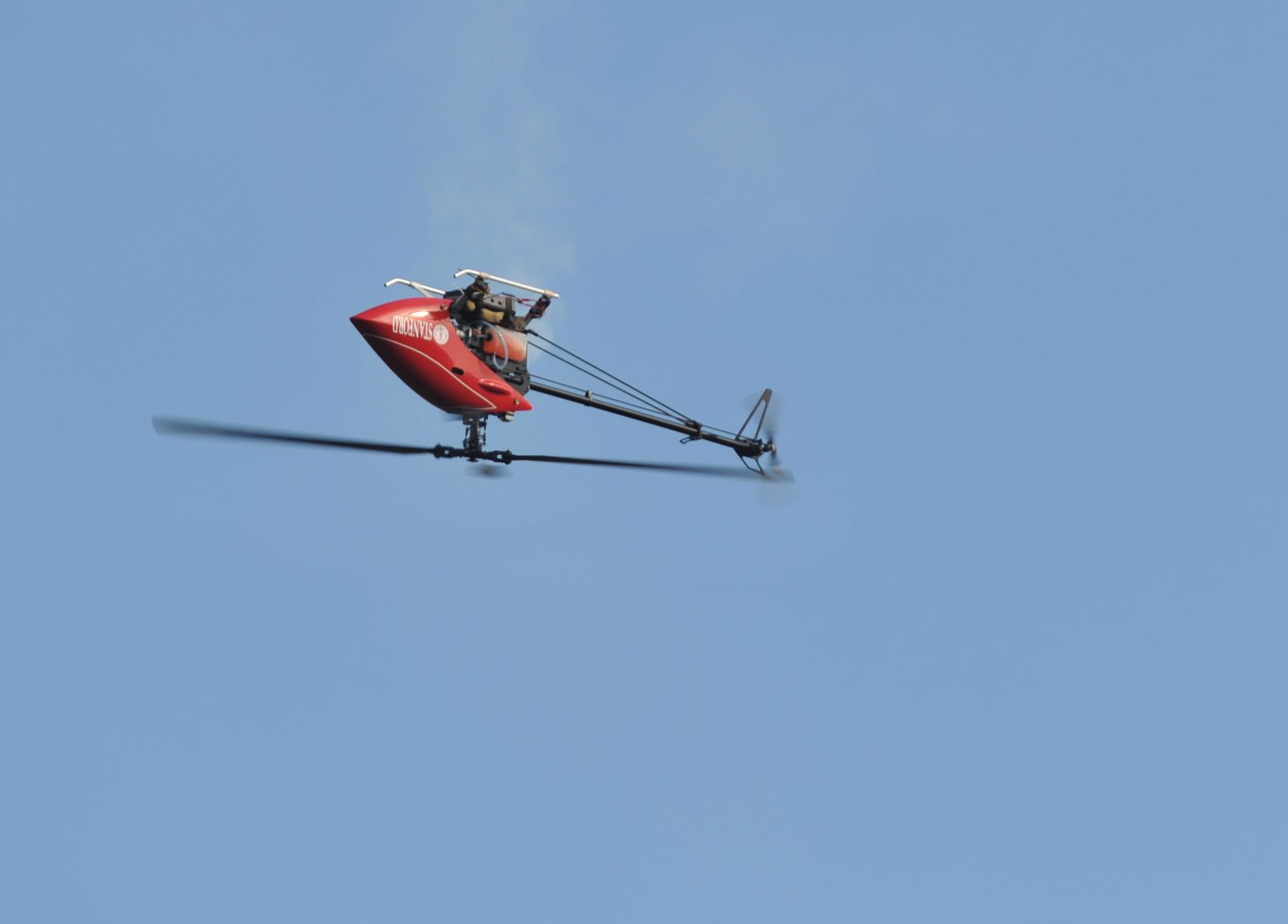
In the early 2000s, this meant focusing on problems like flying helicopters and walking up flights of stairs.

However, there’s still a massive list of problems where humans outperform machines. Although we can no longer claim to beat machines at tasks like Go and image classification, we have a distinct advantage in solving problems that aren’t as well-defined, like judging a well-executed backflip, cleaning a room while preventing accidents, and perhaps the most human problem of all: reasoning about people’s values. Since all these tasks contain some degree of subjectivity, machines need information about the world as well as a way to learn about the people within it in order to solve these problems.

The two tasks of inverse reinforcement learning and apprenticeship learning, formulated almost two decades ago, are closely related to these discrepancies. And solutions to these tasks can be an important step towards our larger goal of learning from humans.

Inverse RL: learning the reward function

In a traditional RL setting, the goal is to learn a decision process to produce behavior that maximizes some predefined reward function. Inverse reinforcement learning (IRL), as described by Andrew Ng and Stuart Russell in 2000^[1], flips the problem and instead attempts to extract the reward function from the observed behavior of an agent.

For example, consider the task of autonomous driving. A naive approach would be to create a reward function that captures the desired behavior of a driver, like stopping at red lights, staying off the sidewalk, avoiding pedestrians, and so on. Unfortunately, this would require an exhaustive list of every behavior we’d want to consider, as well as a list of weights describing how important each behavior is. (Imagine having to decide exactly how much more important pedestrians are than stop signs).

Instead, in the IRL framework, the task is to take a set of human-generated driving data and extract an approximation of that human’s reward function for the task. Of course, this approximation necessarily deals with a simplified model of driving. Still, much of the information necessary for solving a problem is captured within the approximation of the true reward function. As Ng and Russell put it, “the reward function, rather than the policy, is the most succinct, robust, and transferable definition of the task,” since it quantifies how good or bad certain actions are. Once we have the right reward function, the problem is reduced to finding the right policy, and can be solved with standard reinforcement learning methods.

For our self-driving car example, we’d be using human driving data to automatically learn the right feature weights for the reward. Since the task is described completely by the reward function, we do not even need to know the specifics of the human policy, so long as we have the right reward function to optimize. In the general case, algorithms that solve the IRL problem can be seen as a method for leveraging expert knowledge to convert a task description into a compact reward function.

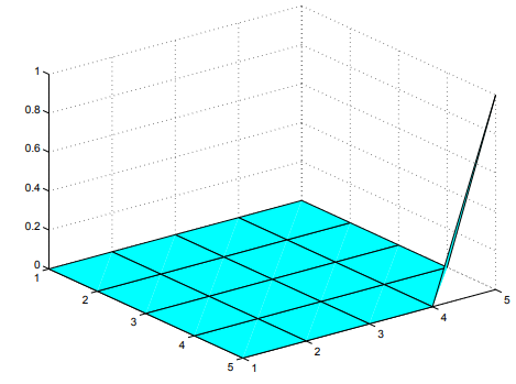
Of course, there’s some nuance here. The main problem when converting a complex task into a simple reward function is that a given policy may be optimal for many different reward functions. That is, even though we have the actions from an expert, there exist many different reward functions that the expert might be attempting to maximize. Some of these functions are just silly: for example, all policies are optimal for the reward function that is zero everywhere, so this reward function is always a possible solution to the IRL problem. But for our purposes, we want a reward function that captures meaningful information about the task and is able to differentiate clearly between desired and undesired policies.

To solve this, Ng and Russell formulate inverse reinforcement learning as an optimization problem. We want to choose a reward function for which the given expert policy is optimal. But given this constraint, we also want to choose a reward function that additionally maximizes certain important properties.

Inverse RL for finite spaces

First, consider the set of optimal policies for a Markov Decision Process (MDP) with a finite state space $S$, set of actions $A$, and transition probability matrices $P_a$ for each action.

In their paper, Ng and Russell proved that a policy $\pi$ given by $\pi(s) \equiv a_1$ is optimal if and only if for all other actions $a$, the reward vector $R$ (which lists the rewards for each possible state) satisfies the condition

$$ (P_{a_1} - P_a)(I - \gamma P_{a_1})^{-1} R \succeq 0. $$

The importance of this theorem is that it shows that we can efficiently select the “best” reward function for which the policy is optimal, using linear programming algorithms. This lets the authors formulate IRL as a tractable optimization problem, where we’re trying to optimize the following heuristics for what makes a reward function “fit” the expert data well:

1. Maximize the difference between the quality of the optimal action and the quality of the next best action (subject to a bound on the magnitude of the reward, to prevent arbitrarily large differences). The intuition here is that we want a reward function that clearly distinguishes the optimal policy from other possible policies.

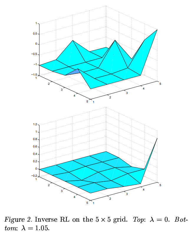
2. Minimize the size of the rewards in the reward function/vector. Roughly speaking, the intuition is that using small rewards encourages the reward function to be simpler, similar to regularization in supervised learning. Ng and Russell choose the L1 norm with an adjustable penalty coefficient, which encourages the reward vector to be non-zero in only a few states.

While these heuristics are intuitive, the authors note that other useful heuristics may exist. In particular, later work, such as Maximum Entropy Inverse Reinforcement Learning (Ziebart et. al.)^[2], and Bayesian Inverse Reinforcement Learning (Ramachandran et. al.)^[3], are two examples of different approaches that build upon the basic IRL framework.

Inverse Reinforcement Learning from Sampled Trajectories

Ng and Russell also describe IRL algorithms for cases where, instead of a full optimal policy, we can only sample trajectories from an optimal policy. That is, we know the states, actions, and rewards generated by a policy for a finite number of episodes, but not the policy itself. This situation is more common in applied cases, especially those dealing with human expert data.

In this formulation of the problem, we replace the reward vector that we used for finite state spaces with a linear approximation of the reward function, which uses a set of feature functions $\phi_i$ to obtain real-valued feature vectors $\phi_i(s)$. These features capture important information from a high-dimensional state space (for instance, instead of storing the location of a car during every time-step, we can store its average speed as a feature). For each feature $\phi_i(s)$ and weight $\alpha_i$ we have:

$$ R(s) = \alpha_1 \phi_1(s) + \alpha_2 \phi_2(s) + \dots + \alpha_d \phi_d(s). $$

and our objective is to find the best-fitting values for each feature-weight $\alpha_i$.

The general idea behind IRL with sampled trajectories is to iteratively improve a reward function by comparing the value of the approximately optimal expert policy with a set of $k$ generated policies. We initialize the algorithm by randomly generating weights for the estimated reward function and initialize our set of candidate policies with a randomly generated policy. Then, the key steps are algorithm are to:

1. Estimate the value of our optimal policy for the initial state $\hat{V}^{\pi}(s_0)$, as well as the value of every generated policy $\hat{V}^{\pi_i}(s_0)$ by taking the average cumulative reward of many randomly sampled trials.

2. Generate an estimate of the reward function $R$ by solving a linear programming problem. Specifically, set $\alpha_i$ to maximize the difference between our optimal policy and each of the other $k$ generated policies.

3. After a large number of iterations, end the algorithm at this step.

4. Otherwise, use a standard RL algorithm to find the optimal policy for $R$. This policy may be different from the given optimal policy, since our estimated reward function is not necessarily identical to the reward function we are searching for.

5. Add the newly generated policy to the set of $k$ candidate policies, and repeat the procedure.

Apprenticeship Learning: learning from a teacher

In addition to learning a reward function from an expert, we can also directly learn a policy to have comparable performance to the expert. This is particularly useful if we have an expert policy that is only approximately optimal. Here, an apprenticeship learning algorithm, formulated by Pieter Abbeel and Andrew Ng in 2004^[4] gives us a solution. This algorithm takes an MDP and an approximately optimal “teacher” policy, and then learns a policy with comparable or better performance to the teacher’s policy using minimal exploration.

This minimal exploration property turns out to be very useful in fragile tasks like autonomous helicopter flight. A traditional reinforcement learning algorithm might start out exploring at random, which would almost certainly lead to a helicopter crash in the first trial. Ideally, we’d be able to use expert data to start with a baseline policy that can be safely improved over time. This baseline policy should be significantly better than a randomly initialized policy, which speeds up convergence.

Apprenticeship learning algorithm

The main idea behind Abbeel and Ng’s algorithm is to use trials from the expert policy to obtain information about the underlying MDP, then iteratively execute a best estimate of the optimal policy for the actual MDP. Executing a policy also gives us data about the transitions in the environment, which we can then use to improve the accuracy of the estimated MDP. Here’s how the algorithm works in a discrete environment:

First, we use the expert policy to learn about the MDP:

1. Run a fixed amount of trials using the expert policy, recording every state-action trajectory.
2. Estimate the transition probabilities for every state-action pair using the recorded data via maximum likelihood estimation.
3. Estimate the value of the expert policy by averaging the total reward in each trial.
   Then, we learn a new policy:
4. Learn an optimal policy for the estimated MDP using any standard reinforcement learning algorithm.
5. Test the learning policy on the actual environment.
6. If performance is not close enough to the value of the expert policy, add the state-action trajectories from this trial to the training set and repeat the procedure to learn a new policy.

The benefit of this method is that at each stage, the policy being tested is the best estimate for the optimal policy of the system. There is diminished exploration, but the core idea of apprenticeship learning is that we can assume the expert policy is already near-optimal.

Further Work

The foundational methods of inverse reinforcement learning and apprenticeship learning, as well as the similar method of imitation learning, are able to achieve their results by leveraging information gleaned from a policy executed by a human expert. However, in the long run, the goal is for machine learning systems to learn from a wide range of human data and perform tasks that are beyond the abilities of human experts.

In particular, when discussing potential avenues for further research in inverse reinforcement learning, Andrew Ng and Stuart Russell highlight suboptimality in the agent’s actions as an important problem. In the context of human experts, it’s clear that while experts may be able to provide a baseline level of performance that RL algorithms could learn from, it will rarely be the case that the expert policy given is actually the optimal one for the environment. The next problem to solve in inverse reinforcement learning would be to extract a reward function without the assumption that the human policy is optimal.

Another remarkable extension to inverse reinforcement learning is one that does not require an optimal policy, and instead considers learning behaviors that agents can identify, but not necessarily demonstrate, meaning that only a classifier is needed. For instance, it’s easy for people to identify whether an agent in a physics simulator is running correctly, but almost impossible to manually specify the right control sequence given the degrees of freedom in a robotics simulator. This extension would allow reinforcement learning systems to achieve human-approved performance without the need for an expert policy to imitate.

The challenge in going from 2000 to 2018 is to scale up inverse reinforcement learning methods to work with deep learning systems. Many recent papers have aimed to do just this — Wulfmeier et al. ^{[5] [6]} use fully convolutional neural networks to approximate reward functions. Finn et al. ^[7] apply neural networks to solve inverse optimal control problems in a robotics context. As these methods improve, inverse reinforcement learning will play an important role in learning policies that are beyond human capability.

---

Citation
For attribution in academic contexts or books, please cite this work as

Jordan Alexander, "Learning from humans: what is inverse reinforcement learning?", The Gradient, 2018.

BibTeX citation:

@article{alexander2018humanreinforcement,
author = {Alexander, Jordan}
title = {Learning from humans: what is inverse reinforcement learning?},
journal = {The Gradient},
year = {2018},
howpublished = {\url{https://thegradient.pub/learning-from-humans-what-is-inverse-reinforcement-learning/ } },
}

---

If you enjoyed this piece and want to hear more, subscribe to the Gradient and follow us on Twitter.

---

1. Ng, Andrew Y., and Stuart J. Russell. "Algorithms for inverse reinforcement learning." ICML. 2000. ↩︎

2. Ziebart, Brian D., et al. "Maximum Entropy Inverse Reinforcement Learning." AAAI. Vol. 8. 2008. ↩︎

3. Ramachandran, Deepak, and Eyal Amir. "Bayesian inverse reinforcement learning." Urbana 51.61801 (2007): 1-4. ↩︎

4. Abbeel, Pieter, and Andrew Y. Ng. "Apprenticeship learning via inverse reinforcement learning." Proceedings of the twenty-first international conference on Machine learning. ACM, 2004. ↩︎

5. Wulfmeier, Markus, Peter Ondruska, and Ingmar Posner. "Maximum entropy deep inverse reinforcement learning." arXiv preprint arXiv:1507.04888 (2015). ↩︎

6. Wulfmeier, Markus, et al. "Large-scale cost function learning for path planning using deep inverse reinforcement learning." The International Journal of Robotics Research 36.10 (2017): 1073-1087. ↩︎

7. Finn, Chelsea, Sergey Levine, and Pieter Abbeel. "Guided cost learning: Deep inverse optimal control via policy optimization." International Conference on Machine Learning. 2016. ↩︎