Neural algorithmic reasoning

In this article, we will talk about classical computation: the kind of computation typically found in an undergraduate Computer Science course on Algorithms and Data Structures [1]. Think shortest path-finding, sorting, clever ways to break problems down into simpler problems, incredible ways to organise data for efficient retrieval and updates. Of course, given The Gradient’s focus on Artificial Intelligence, we will not stop there; we will also investigate how to capture such computation with deep neural networks.

Why capture classical computation?

Maybe it’s worth starting by clarifying where my vested interest in classical computation comes from. Competitive programming—the art of solving problems by rapidly writing programs that need to terminate in a given amount of time, and within certain memory constraints—was a highly popular activity in my secondary school. For me, it was truly the gateway into Computer Science, and I trust the story is similar for many machine learning practitioners and researchers today. I have been able to win several medals at international programming competitions, such as the Northwestern Europe Regionals of the ACM-ICPC, the top-tier Computer Science competition for university students. Hopefully, my successes in competitive programming also give me some credentials to write about this topic.

While this should make clear why I care about classical computation, why should we all care? To arrive at this answer, let us ponder some of the key properties that classical algorithms have:

• They are provably correct, and we can often have strong guarantees about the resources (time or memory) required for the computation to terminate.
• They offer strong generalisation: while algorithms are often devised by observing several small-scale example inputs, once implemented, they will work without fault on inputs that are significantly larger, or distributionally different than such examples.
• By design, they are interpretable and compositional: their (pseudo)code representation makes it much easier to reason about what the computation is actually doing, and one can easily recompose various computations together through subroutines to achieve different capabilities.

Looking at all of these properties taken together, they seem to be exactly the issues that plague modern deep neural networks the most: you can rarely guarantee their accuracy, they often collapse on out-of-distribution inputs, and they are very notorious as black boxes, with compounding errors that can hinder compositionality.

However, it is exactly those skills that are important for making AI instructive and useful to humans! For example, to have an AI system that reliably and instructively teaches a concept to a human, the quality of its output should not depend on minor details of the input, and it should be able to generalise that concept to novel situations. Arguably, these skills are also a missing key step on the road to building generally-intelligent agents. Therefore, if we are able to make any strides towards capturing traits of classical computation in deep neural networks, this is likely to be a very fruitful pursuit.

First impressions: Algorithmic alignment

My journey into the field started with an interesting, but seemingly inconsequential question:

Can neural networks learn to execute classical algorithms?

This can be seen as a good way to benchmark to what extent are certain neural networks capable of behaving algorithmically; arguably, if a system can produce the outputs of a certain computation, it has “captured” it. Further, learning to execute provides a uniquely well-built environment for evaluating machine learning models:

• An infinite data source—as we can generate arbitrary amounts of inputs;
• They require complex data manipulation—making it a challenging task for deep learning;
• They have a clearly specified target function—simplifying interpretability analyses.

When we started studying this area in 2019, we really did not think more of it than a very neat benchmark—but it was certainly becoming a very lively area. Concurrently with our efforts, a team from MIT tried tackling a more ambitious, but strongly related problem:

What makes a neural network better (or worse) at fitting certain (algorithmic) tasks?

The landmark paper, “What Can Neural Networks Reason About?” [2] established a mathematical foundation for why an architecture might be better for a task (in terms of sample complexity: the number of training examples needed to reduce validation loss below epsilon). The authors’ main theorem states that better algorithmic alignment leads to better generalisation. Rigorously defining algorithmic alignment is out of scope of this text, but it can be very intuitively visualised:

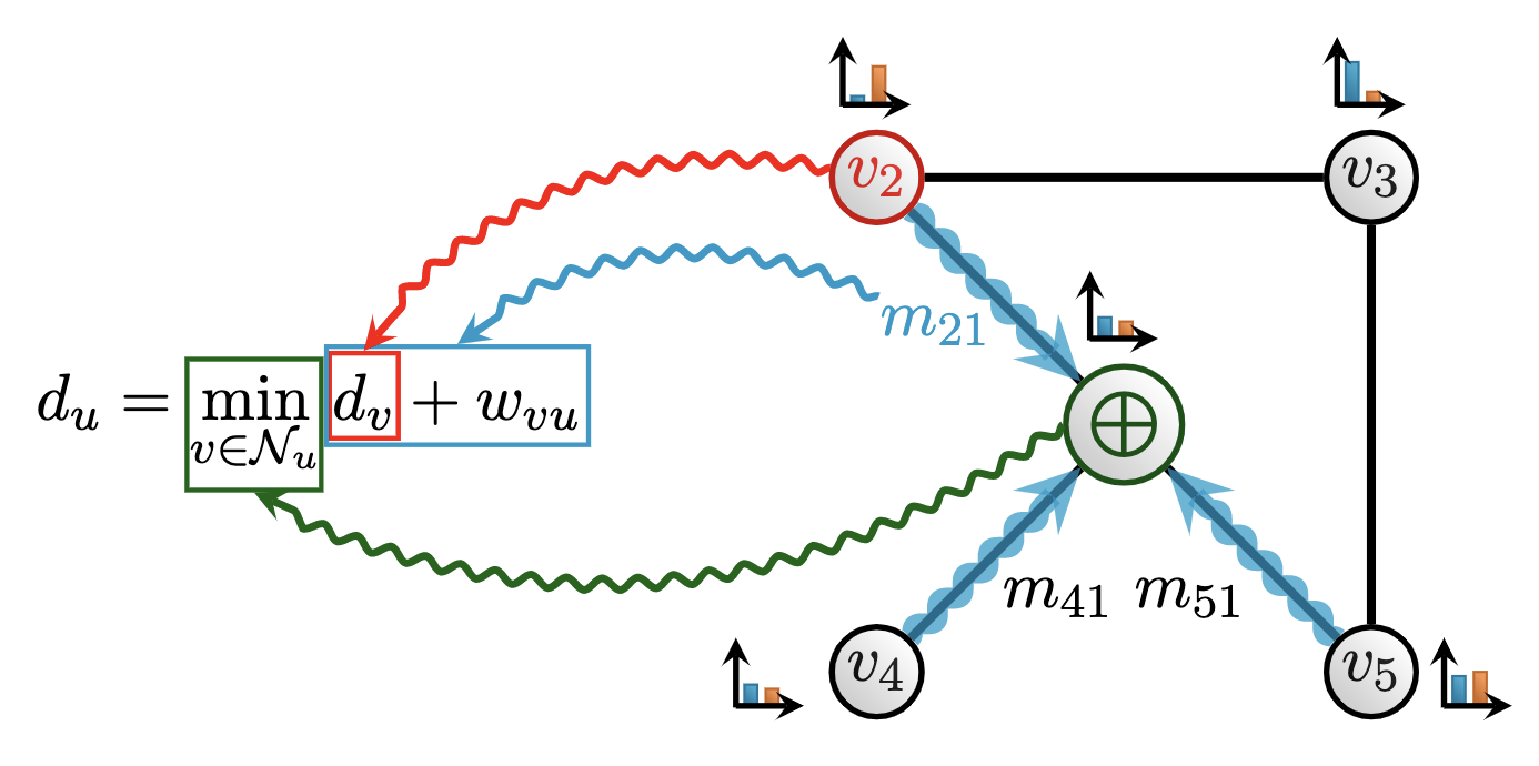
Here, we can see a visual decomposition of how a graph neural network (GNN) [3] aligns with the classical Bellman-Ford [4] algorithm for shortest path-finding. Specifically, Bellman-Ford maintains its current estimate of how far away each node is from the source node: a distance variable (du) for each node u in a graph. At every step, for every neighbour v of node u, an update to du is proposed: a combination of (optimally) reaching v, and then traversing the edge connecting v and u (du + wvu). The distance variable is then updated as the optimal out of all the proposals. Operations of a graph neural network can naturally decompose to follow the data flow of Bellman-Ford:

• The distance variables correspond to the node features maintained by the GNN;
• Adding the edge distance to a distance variable corresponds to computing the GNN’s message function;
• Choosing the optimal neighbour based on this measure corresponds to the GNN’s permutation-invariant aggregation function, ⨁.

Generally, it can be proven that, the more closely we can decompose our neural network to follow the algorithm’s structure, the more favourable sample complexity we can expect when learning to execute such algorithms. Bellman-Ford is a typical instance of a dynamic programming (DP) algorithm [5], a general-purpose problem-solving strategy that breaks the problem down into subproblems, and then recombines their solutions to find the final solution.

The MIT team made the important observation that GNNs appear to algorithmically align with DP, and since DP can itself be used to express many useful forms of classical computation, GNNs should be a very potent general-purpose model for learning to execute. This was validated by several carefully constructed DP execution benchmarks, where relational models like GNNs clearly outperformed architectures with weaker inductive biases. GNNs have been a long-standing interest of mine [6], so the time was right to release our own contribution to the area:

Neural Execution of Graph Algorithms

In this paper [7], concurrently released with Xu et al. [2], we conducted a thorough empirical analysis of learning to execute with GNNs. We found that while algorithmic alignment is indeed a powerful tool for model class selection, it unfortunately does not allow us to be reckless. Namely, we cannot just apply any expressive GNN to an algorithmic execution task and expect great results, especially out-of-distribution—which we previously identified as a key setting in which “true” reasoning systems should perform well. Much like other neural networks, GNNs can very easily overfit to the characteristics of the distribution of training inputs, learning “clever hacks” and sidestepping the actual procedure that they are attempting to execute.

We hence identify three key observations on careful inductive biases to use, to improve the algorithmic alignment to certain path-finding problems even further and allow for generalising to 5x larger inputs at test time:

1. Most traditional deep learning setups involve a stack of layers with unshared parameters. This fundamentally limits the amount of computation the neural network can perform: if, at test time, an input much larger than the ones in the training data arrives, it would be expected that more computational steps are needed—yet, the unshared GNN has no way to support that. To address this, we adopt the encode-process-decode paradigm [8]: a single shared processor GNN is iterated for many steps, and this number of steps can be variable at both training and inference time. Such an architecture also allows a neat way to algorithmically align to iterative computation, as most algorithms involve repeatedly applying a certain computation until convergence.
2. Since most path-finding algorithms (including Bellman-Ford) require “local” optimisation (i.e. choosing exactly one optimal neighbour at every step), we opted to use max aggregation to combine the messages sent in GNNs. While this may seem like a very intuitive idea, it went strongly against the folklore of the times, as max-GNNs were known to be theoretically inferior to sum-GNNs at distinguishing non-isomorphic graphs [9]. (We now have solid theoretical evidence [10] for why this is a good idea.)
3. Lastly, while most deep learning setups only require producing an output given an input, we found that this misses out on a wealth of ways to instruct the model to align to the algorithm. For example, there are many interesting invariants that algorithms have that can be explicitly taught to a GNN. In the case of Bellman-Ford, after k iterations are executed, we should be expected to be able to recover all shortest paths that are no more than k hops away from the source node. Accordingly, we use this insight to provide step-wise supervision to the GNN at every step. This idea appears to be gaining traction in Large Language Model design in recent months [11, 12].

All three of the above changes make for stronger algorithmically-aligned GNNs.

Playing the alignment game

It must be stressed that the intuitive idea of algorithmic alignment—taking inspiration from Computer Science concepts in architecture design—is by no means novel! The text-book example of this are the neural Turing machine (NTM) and differentiable neural computer (DNC) [13, 14]. These works are decisively influential; in fact, in its attempt to make random-access memory compatible with gradient-based optimisation, the NTM gave us one of the earliest forms of content-based attention, three years before Transformers [15]!

However, despite their influence, these architectures are nowadays virtually never used in practice. There are many possible causes for this, but in my opinion it is because their design was too brittle: trying to introduce many differentiable components into the same architecture at once, without a clear guidance on how to compose them, or a way to easily debug them once they failed to show useful signal on a new task. Our line of work still wants to build something like an NTM—but make it more successfully deployed, by using algorithmic alignment to more carefully prototype each building block in isolation, and have a more granular view of which blocks benefit execution of which target algorithms.

Our approach of “playing the algorithmic alignment game” appears to have yielded a successful line of specialised (G)NNs, and we now have worthy ‘fine-grained’ solutions for learning to execute linearithmic sequence algorithms [16], iterative algorithms [17], pointer-based data structures [18], as well as persistent auxiliary memory [19]. Eventually, these insights also carried over to more fine-grained theory as well. In light of our NEGA paper [7], the inventors of algorithmic alignment refined their theory into what is now known as linear algorithmic alignment [10], providing justification for, among other things, our use of the max aggregation. More recent insights show that understanding algorithmic alignment may require causal reasoning [20,21], properly formalising it may require category theory [22], and properly describing it may require analysing asynchronous computation [23]. Algorithmic alignment is therefore turning into a very exciting area for mathematical approaches to deep learning in recent years.

Why not just run the target algorithm?...and rebuttals

While it appears a lot of useful progress has been made towards addressing our initial “toy question”, the idea of learning to execute is not one that easily passes peer review. My personal favourite reviewer comment I received—quoted in full—was as follows: “This paper will certainly accelerate research in building algorithmic models, and there’s certainly a lot of researchers that would make advantage of it, I am just not sure that this research should even exist”.

This is clearly not the nicest thing to receive as the first author of a paper. But still, let’s try to put my ego aside, and see what can be taken away from such reviews. There is a clear sense in which such reviews are raising an entirely valid point: tautologically, the target algorithm will execute itself better (or equally good) than any GNN we’d ever learn over it. Clearly, if we want wide-spread recognition of these ideas, we need to show how learning to execute can be usefully applied beyond the context of “pure” execution.

Our exploration led us to many possible ideas, and in the remainder of this article, I will show three ideas that saw the most impact.

First, algorithmically aligned models can accelerate science. And if you want clear evidence of this, look no further than the cover of Nature [24]. In our work, we train (G)NNs to fit a mathematical dataset of interest to a mathematician, and then use simple gradient saliency methods to signal to the mathematician which parts of the inputs to focus their attention at. While such signals are often remarkably noisy, they do allow a mathematician to study only the most salient 20-30 nodes in a graph that would otherwise have hundreds or thousands of nodes, making pattern discovery much easier. The discovered patterns can then form the basis of novel theorems, and/or be used to derive conjectures.

With this simple approach, we were able to drive independent contributions to two highly disparate areas of math: knot theory [25] and representation theory [26], both subsequently published in their areas’ respective top-tier journals, hence earning us the Nature accolade. But, while our approach is simple in principle, a question arose especially in the representation theory branch: which (G)NN to use? Standard expressive GNNs did not yield clearly interpretable results.

This is where algorithmic alignment helped us: Geordie Williamson, our representation theory collaborator, provided an algorithm that would compute the outputs we care about, if we had access to privileged information. We achieved our best results with a GNN model that was explicitly aligning its components to this target algorithm.

More generally: in this case, a target algorithm existed, but executing it was inapplicable (due to privileged inputs). Algorithmic alignment allowed us to embed “priors” from it anyway.

Second, algorithmically aligned models are fast heuristics. In recent work with computer networking and machine learning collaborators from ETH Zürich, we studied the applicability of neural algorithmic reasoning in computer networking [27]. Specifically, we sought to expedite the challenging task of configuration synthesis: based on a given specification of constraints a computer network should satisfy, produce a corresponding network configuration (a graph specifying the routers in a network and their connections). This configuration must satisfy all of the specifications, once a network protocol has been executed over it.

Producing these configurations is known to be a very challenging NP-hard problem—in practice, it is usually solved with slow SMT solvers, which can often require doubly-exponential complexity. Instead, we choose to use ideas from algorithmic reasoning to generate configurations by inverting the protocol (which can be seen as a graph algorithm). Specifically, we generate many random network configurations, execute the protocol over them, and collect all true facts about the resulting network to extract corresponding specifications. This gives us all we need to generate a graph-based dataset from specifications to configurations, and fit an algorithmically-aligned GNN to this dataset.

Naturally, by virtue of just requiring a forward pass of a machine learning model, this approach is substantially faster than SMT solvers at inference time: for certain configurations, we have observed over 490x speedup over the prior state-of-the-art. Of course, there is no free lunch: the price we pay for this speedup are occasional inaccuracies in the produced configurations at test-time. That being said, on all the relevant distributions we evaluated, the average number of constraints satisfied has consistently been over 90%, which makes our method already applicable for downstream human-in-the-loop use—and it is likely to accelerate human designers, as very often, the initial configurations are unsatisfiable, meaning SMT solvers will spend a lot of effort only to say a satisfying configuration cannot be found. During this time, a fast forward pass of a GNN could have allowed for far more rapid iteration.

More generally: in this case, a target algorithm is only being approximated, but such that it provides a fast and reasonably accurate heuristic, enabling rapid human-in-the-loop iteration.

A core problem with applying classical algorithms

To set us up for the third and final idea, let me pose a motivating task: “Find me the optimal path from A to B”. How do you respond to this prompt?

Chances are, especially if you come from a theoretical Computer Science background like me, that you will respond to this question in a very singular way. Namely, you will subtly assume that I am providing you with a weighted graph and asking you for the shortest path between two specific vertices in this graph. We can then diligently apply our favourite path-finding algorithm (e.g. Dijkstra’s algorithm [28]) to resolve this query. I should highlight that, at least at the time of writing this text, the situation is not very different with most of today’s state-of-the-art AI chatbots—when prompted with the above task, while they will often seek further information, they will promptly assume that there is an input weighted graph provided!

However, there’s nothing in my question that requires either of these assumptions to be true. Firstly, the real-world is often incredibly noisy and dynamic, and rarely provides such abstractified inputs. For example, the task might concern the optimal way to travel between two places in a real-world transportation network, which is a challenging routing problem that relies on processing noisy, complex data to estimate real-time traffic speeds—a lesson I’ve personally learnt, when I worked on deploying GNNs within Google Maps [29]. Secondly, why must “optimal” equal shortest? In the context of routing traffic, and depending on the specific contexts and goals, “optimal” may well mean most cost-efficient, least polluting, etc. All of these variations make a straightforward application of Dijkstra’s algorithm difficult, and may in practice require a combination of several algorithms.

Both of these issues highlight that we often need to make a challenging mapping between complex real-world data and an input that will be appropriate for running a target algorithm. Historically, this mapping is performed by humans, either manually or via specialised heuristics. This naturally invites the following question: Can humans ever hope to be able to manually find the necessary mapping, in general? I would argue that, at least since the 1950s, we’ve known the answer to this question to be no. Directly quoting from the paper of Harris and Ross [30], which is one of the first accounts of the maximum flow problem (through analysing railway networks):

The evaluation of both railway system and individual track capacities is, to a considerable extent, an art. The authors know of no tested mathematical model or formula that includes all variations and imponderables that must be weighed. Even when the individual has been closely associated with the particular territory he is evaluating, the final answer, however accurate, is largely one of judgment and experience.

Hence, even highly skilled humans often need to make educated guesses when attaching a single scalar “capacity” value to each railway link—and this needs to be done before any flow algorithm can be executed over the input network! Furthermore, as evidenced by the following statement from the recent Amazon Last Mile Routing Research Challenge [31],

...there remains an important gap between theoretical route planning and real-life route execution that most optimization-based approaches cannot bridge. This gap relates to the fact that in real-life operations, the quality of a route is not exclusively defined by its theoretical length, duration, or cost but by a multitude of factors that affect the extent to which drivers can effectively, safely, and conveniently execute the planned route under real-life conditions.

Hence, these considerations remain relevant even in the high-stakes, big data settings of today. This is a fundamental divide between classical algorithms and the real-world problems they were originally designed to solve! Satisfying the strict preconditions for applying an algorithm may lead to drastic loss of information from complex, naturally-occurring inputs. Or, put simply:

It doesn’t matter if the algorithm is provably correct, if we execute it on the wrong inputs!

This issue gets significantly tricker if the data is partially observable, there are adversarial actors in the environment, etc. I must stress that this is not an issue theoretical computer scientists tend to concern themselves with, and probably for good reason! Focussing on the algorithms in the “abstractified” setting is already quite challenging, and it has yielded some of the most beautiful computational routines that have significantly transformed our lives. That being said, if we want to give “superpowers” to these routines and make them applicable way beyond the kinds of inputs they were originally envisioned for, we need to find some way to bridge this divide. Our proposal, the neural algorithmic reasoning blueprint [32], aims to bridge this divide by neuralising the target algorithm.

Neural Algorithmic Reasoning

Since a key limitation we identified is the need for manual input feature engineering, a good first point of attack could be to simply replace the feature engineer with a neural network encoder. After all, replacing feature engineering is how deep learning got its major breakthrough [33]! The encoder would learn to predict the inputs to the algorithm from the raw data, and then we can execute the algorithm over these inputs to obtain the outputs we care about.

This kind of pipeline is remarkably popular [34]; in recent times, there have been seminal results allowing for backpropagating through the encoder even when the algorithm itself is non-differentiable [35]. However, it suffers from an algorithmic bottleneck problem: namely, it is fully committing itself to the algorithm’s outputs [36]. That is, if the inputs to the algorithm are poorly predicted by the encoder, we run into the same issue as before—the algorithm will give a perfect answer in an incorrect environment. Since the required inputs are usually scalar in nature (e.g. a single distance per edge of the input graph), the encoder is often tasked with mapping the extremely rich structure of real world data into only a single number. This particularly becomes an issue with low-data or partially-observable scenarios.

To break the algorithmic bottleneck, we instead opt to represent both the encoder and the algorithm as high-dimensional neural networks! Now, our algorithmic model is a processor neural network—mapping high dimensional embeddings to high dimensional embeddings. To recover relevant outputs, we can then attach an appropriate decoder network to the output embeddings of the processor. If we were able to guarantee that this processor network “captures the computation” of the algorithm, then we would simultaneously resolve all of the issues previously identified:

• Our pipeline would be an end-to-end differentiable neural network;
• It would also be high-dimensional throughout, alleviating the algorithmic bottleneck;
• If any computation can not be explained by the processor, we can add skip connections going directly from the encoder to the decoder, to handle such residual information.

So, all we need now is to produce a neural network which captures computation! But, wait… that’s exactly what we have been talking about in this entire blog post! :)

We have arrived at the neural algorithmic reasoning (NAR) blueprint [32]:

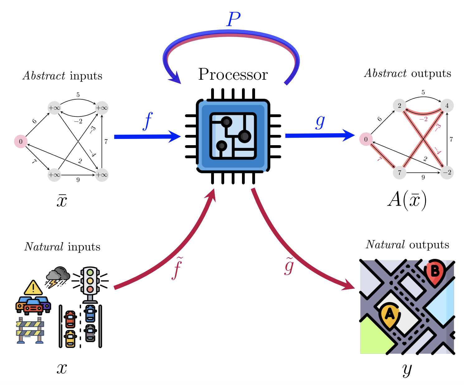
This figure represents a neat summary of everything we have covered so far: first, we obtain a suitable processor network, P, by algorithmic alignment to a target algorithm, or pre-training on learning to execute the target algorithm, or both! Once ready, we include P into any neural pipeline we care about over raw (natural) data. This allows us to apply target algorithms “on inputs previously considered inaccessible to them”, in the words of the original NAR paper [32]. Depending on the circumstances, we may or may not wish to keep P’s parameters frozen once deployed, or P may even be entirely nonparametric [37,38]!

While initially only a proposal, there are now several successful NAR instances that have been published at top-tier venues [36,39,40,41]. In the most-recent such paper [41], we aimed to study how to classify blood vessels in the mouse brain—a very challenging graph task spanning millions of nodes and edges [42]. However, while it’s not trivial to directly classify blood vessels from their features, it is reasonably safe to assume that the main purpose of blood vessels is to conduct blood flow—hence, an algorithm for flow analysis could be a suitable one to deploy here. Accordingly, we first pre-trained a NAR processor to execute the relevant maximum-flow and minimum-cut algorithms [43], then successfully deployed it on the brain vessel graph, surpassing the previous state-of-the-art GNNs. It is worthy to note that the brain vessel graph is 180,000x larger than the synthetic graphs we used for learning to execute, and minimal hyperparameter tuning was applied throughout! We are confident this success is only the first of many.

Where can we get good processors from?

While the ideas given in prior subsections hopefully provide a good argument for the utility of capturing classical computation, in practice we still need to know which computation to capture! All of the NAR papers referenced above use target algorithms highly relevant to the downstream task, and the processors are trained using bespoke execution datasets built on top of those algorithms. This often requires both domain expertise and computer science expertise, and hence represents a clear barrier of entry!

Since my beginnings in NAR, I have been strongly interested in reducing this barrier of entry, while also providing a collection of “base processors” that should be useful in a wide variety of tasks. This resulted in a two-year-long engineering effort, culminating by open-sourcing the CLRS Algorithmic Reasoning Benchmark (https://github.com/deepmind/clrs) [44].

The CLRS benchmark was inspired by the iconic Introduction to Algorithms (CLRS) textbook from Cormen, Leiserson, Rivest and Stein [1], which is one of the most popular undergraduate textbooks on classical algorithms and data structures, and a “bible” for competitive programmers. Despite its many thousands of pages, it only contains ~90 distinct algorithms, and these algorithms tend to form the foundations behind entire careers in software engineering! Hence, the algorithms in CLRS can form our desired solid set of “base processors”, and we set out to make it easy to construct and train NAR processors to execute the algorithms in CLRS.

In its first incarnation, we released CLRS-30, a collection of dataset and processor generators for thirty algorithms in CLRS, spanning a wide variety of skills: sorting, searching, dynamic programming, graph algorithms, string algorithms and geometric algorithms.

What makes CLRS-30 special is the wide variety of data, models and pipelines it exposes to the user: given an appropriate specification of the target algorithm’s variables, an implementation of the target algorithm, and a desirable random input sampler, CLRS will automatically produce the full execution trajectories of this algorithm’s variables in a spatio-temporal graph-structured format, relevant encoder/decoder/processor models, and loss functions. For this reason, we typically refer to CLRS as a “dataset and baseline generator” rather than an individual dataset.

For example, here is a CLRS-produced trajectory for insertion sorting a list [5, 2, 4, 3, 1]:

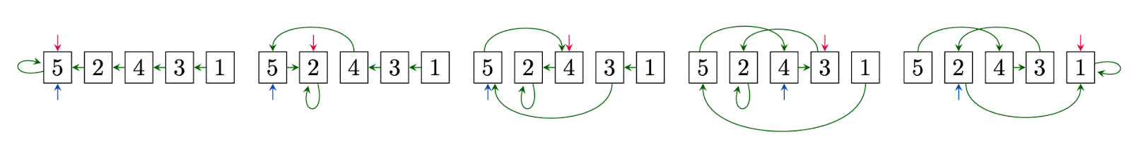
This trajectory fully exposes the internal state of the algorithm: how the list’s pointers (in green) change over time, which element is currently being sorted (in red), and the position it needs to be sorted into (in blue). By default, these can be used for step-wise supervision, although recently more interesting ways to use the trajectories, such as Hint-ReLIC [21], were proposed.

Why stop at just one algorithm? Could we learn all thirty?

As mentioned, CLRS-30 converts thirty diverse algorithms into a unified graph representation. This paves the way for an obvious question: could we learn one processor (with a single set of weights) to execute all of them? To be clear, we envision a NAR processor like this:

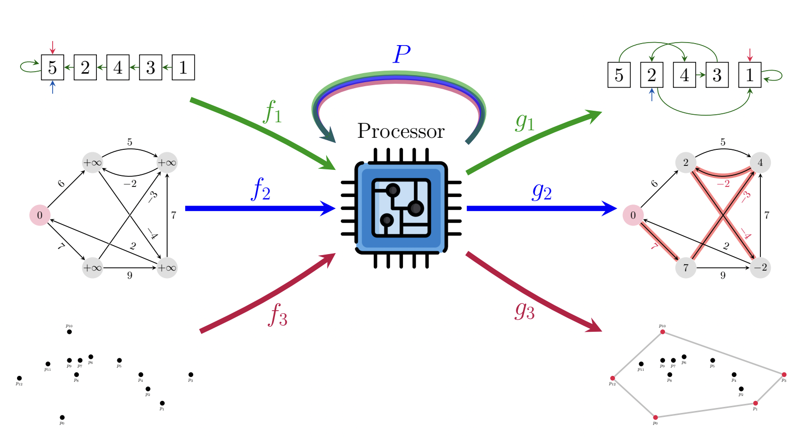
That is, a single (G)NN, capable of executing sorting, path-finding, convex hull finding, and all other CLRS algorithms. Since the input and output dimensionalities can vary wildly between the different algorithms, we would still propose using separate encoders and decoders for each algorithm—mapping into and out of the processor’s latent space—however, we deliberately keep these as linear functions to place the majority of the computational effort on P.

However, despite the base idea being simple in principle, this proves to be no trivial endeavour. Most prior attempts to learn multiple algorithms, such as NEGA [7] or its successor, NE++ [45], have deliberately focussed on learning to execute highly related algorithms, where the learning signals are likely to be well-correlated. Accordingly, our initial single-processor multi-task training runs on all of CLRS-30 resulted in NaNs.

We have been able to identify single-task instabilities as the main culprit of this: if the gradients for any individual algorithmic task are noisy or unstable, this translates to unstable training on all thirty of them. Hence, we launched a dedicated “mini-strike” of two months to identify and fix learning stability issues in single-task learners. Our resulting model, Triplet-GMPNN [46], improves absolute mean performance over CLRS-30 by over 20% from prior state-of-the-art, and enables successful multi-task training! What’s more, we now have a single generalist Triplet-GMPNN that, on average, matches the thirty specialist Triplet-GMPNNs, evaluated out-of-distribution:

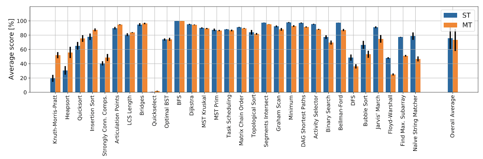
While it is evident from this plot that we still have a long way to go before we produce a fully “algorithmic” NAR processor library, this result has been seen as a significant “compression” milestone, similar to the Gato [47] paper. The release of our Triplet-GMPNN model sparked extremely interesting discussions on Twitter, Reddit and HackerNews, especially in light of its implications to constructing generally-intelligent systems.  Generally, the progress in NAR made by various groups over just the past three years has been incredible to observe. And we’re just getting started: now that we can, in principle, build generalist NAR processors, I am immensely excited about the potential this holds for future research and products.

Want to know more?

Needless to say, there is a lot of material this article does not cover—especially, the technical and implementation details of many of the papers discussed herein. If what you’ve read here has made you interested to know more, or even play with NAR models yourself, I recommend you check out the LoG’22 Tutorial on NAR (https://algo-reasoning.github.io/), which I delivered alongside Andreea Deac and Andrew Dudzik. Over the course of just under three hours, we cover all of the theory needed to master the foundations of developing, deploying, and deepening neural algorithmic reasoners, along with plentiful code pointers and references. And of course, you are more than welcome to reach out directly, should you have any follow-up questions, interesting points of discussion, or even interesting ideas for projects!

References

1. TH. Cormen, CE. Leiserson, RL. Rivest, and C. Stein. Introduction to Algorithms. MIT Press’22.
2. K. Xu, J. Li, M. Zhang, SS. Du, K-I. Kawarabayashi, and S. Jegelka. What Can Neural Networks Reason About?. ICLR’20.
3. P. Veličković. Everything is Connected: Graph Neural Networks. Current Opinion in Structural Biology’23.
4. R. Bellman. On a Routing Problem. Quarterly of Applied Mathematics’58.
5. R. Bellman. Dynamic Programming. Science’66.
6. P. Veličković, G. Cucurull, A. Casanova, A. Romero, P. Liò, and Y. Bengio. Graph Attention Networks. ICLR’18.
7. P. Veličković, R. Ying, M. Padovano, R. Hadsell, and C. Blundell. Neural Execution of Graph Algorithms. ICLR’20.
8. JB. Hamrick, KR. Allen, V. Bapst, T. Zhu, KR. McKee, JB. Tenenbaum, and PW. Battaglia. Relational inductive biases for physical construction in humans and machines. CCS’18.
9. K. Xu*, W. Hu*, J. Leskovec, and S. Jegelka. How Powerful are Graph Neural Networks?. ICLR’19.
10. K. Xu, M. Zhang, J. Li, SS. Du, K-I. Kawarabayashi, and S. Jegelka. How Neural Networks Extrapolate: From Feedforward to Graph Neural Networks. ICLR’21.
11. J. Uesato*, N. Kushman*, R. Kumar*, F. Song, N. Siegel, L. Wang, A. Creswell, G. Irving, and I. Higgins. Solving math word problems with process- and outcome-based feedback. arXiv’22.
12. H. Lightman*, V. Kosaraju*, Y. Burda*, H. Edwards, B. Baker, T. Lee, J. Leike, J. Schulman, I. Sutskever, and K. Cobbe. Let’s Verify Step by Step. arXiv’23.
13. A. Graves, G. Wayne, and I. Danihelka. Neural Turing Machines. arXiv’14.
14. A. Graves, G. Wayne, M. Reynolds, T. Harley, I. Danihelka, A. Grabska-Barwińska, S. Gómez Colmenarejo, E. Grefenstette, T. Ramalho, J. Agapiou, A. Puigdomènech Badia, KM. Hermann, Y. Zwols, G. Ostrovski, A. Cain, H. King, C. Summerfield, P. Blunsom, K. Kavukcuoglu, and D. Hassabis. Hybrid computing using a neural network with dynamic external memory. Nature’16.
15. A. Vaswani*, N. Shazeer*, N. Parmar*, J. Uszkoreit*, L. Jones*, AN. Gomez*, Ł. Kaiser*, and I. Polosukhin*. Attention is all you need. NeurIPS’17.
16. K. Freivalds, E. Ozoliņš, and A. Šostaks. Neural Shuffle-Exchange Networks - Sequence Processing in O(n log n) Time. NeurIPS’19.
17. H. Tang, Z. Huang, J. Gu, B-L. Lu, and H. Su. Towards Scale-Invariant Graph-related Problem Solving by Iterative Homogeneous GNNs. NeurIPS’20.
18. P. Veličković, L. Buesing, MC. Overlan, R. Pascanu, O. Vinyals, and C. Blundell. Pointer Graph Networks. NeurIPS’20.
19. H. Strathmann, M. Barekatain, C. Blundell, and P. Veličković. Persistent Message Passing. ICLR’21 SimDL.
20. B. Bevilacqua, Y. Zhou, and B. Ribeiro. Size-invariant graph representations for graph classification extrapolations. ICML’21.
21. B. Bevilacqua, K. Nikiforou*, B. Ibarz*, I. Bica, M. Paganini, C. Blundell, J. Mitrovic, and P. Veličković. Neural Algorithmic Reasoning with Causal Regularisation. ICML’23.
22. A. Dudzik*, and P. Veličković*. Graph Neural Networks are Dynamic Programmers. NeurIPS’22.
23. A. Dudzik, T. von Glehn, R. Pascanu, and P. Veličković. Asynchronous Algorithmic Alignment with Cocycles. ICML’23 KLR.
24. A. Davies, P. Veličković, L. Buesing, S. Blackwell, D. Zheng, N. Tomašev, R. Tanburn, P. Battaglia, C. Blundell, A. Juhász, M. Lackenby, G. Williamson, D. Hassabis, and P. Kohli. Advancing mathematics by guiding human intuition with AI. Nature’21.
25. A. Davies, A. Juhász, M. Lackenby, and N. Tomašev. The signature and cusp geometry of hyperbolic knots. Geometry & Topology (in press).
26. C. Blundell, L. Buesing, A. Davies, P. Veličković, and G. Williamson. Towards combinatorial invariance for Kazhdan-Lusztig polynomials. Representation Theory’22.
27. L. Beurer-Kellner, M. Vechev, L. Vanbever, and P. Veličković. Learning to Configure Computer Networks with Neural Algorithmic Reasoning. NeurIPS’22.
28. EW. Dijkstra. A note on two papers in connection with graphs. Numerische Matematik’59.
29. A. Derrow-Pinion, J. She, D. Wong, O. Lange, T. Hester, L. Perez, M. Nunkesser, S. Lee, X. Guo, B. Wiltshire, PW. Battaglia, V. Gupta, A. Li, Z. Xu, A. Sanchez-Gonzalez, Y. Li, and P. Veličković. ETA Prediction with Graph Neural Networks in Google Maps. CIKM’21.
30. TE. Harris, and FS. Ross. Fundamentals of a method for evaluating rail net capacities. RAND Tech Report’55.
31. M. Winkenbach, S. Parks, and J. Noszek. Technical Proceedings of the Amazon Last Mile Routing Research Challenge. 2021.
32. P. Veličković, and C. Blundell. Neural Algorithmic Reasoning. Patterns’21.
33. A. Krizhevsky, I. Sutskever, and GE. Hinton. ImageNet Classification with Deep Convolutional Neural Networks. NeurIPS’12.
34. Q. Cappart, D. Chételat, EB. Khalil, A. Lodi, C. Morris, and P. Veličković. Combinatorial optimization and reasoning with graph neural networks. JMLR’23.
35. M. Vlastelica*, A. Paulus*, V. Musil, G. Martius, and M. Rolínek. Differentiation of Blackbox Combinatorial Solvers. ICLR’20.
36. A. Deac, P. Veličković, O. Milinković, P-L. Bacon, J. Tang, and M. Nikolić. Neural Algorithmic Reasoners are Implicit Planners. NeurIPS’21.
37. B. Wilder, E. Ewing, B. Dilkina, and M. Tambe. End to end learning and optimization on graphs. NeurIPS’19.
38. M. Garnelo, and WM. Czarnecki. Exploring the Space of Key-Value-Query Models with Intention. 2023.
39. Y. He, P. Veličković, P. Liò, and A. Deac. Continuous Neural Algorithmic Planners. LoG’22.
40. P. Veličković*, M. Bošnjak*, T. Kipf, A. Lerchner, R. Hadsell, R. Pascanu, and C. Blundell. Reasoning-Modulated Representations. LoG’22.
41. D. Numeroso, D. Bacciu, and P. Veličković. Dual Algorithmic Reasoning. ICLR’23.
42. JC. Paetzold, J. McGinnis, S. Shit, I. Ezhov, P. Büschl, C. Prabhakar, MI. Todorov, A. Sekuboyina, G. Kaissis, A. Ertürk, S. Günnemann, and BH. Menze. Whole Brain Vessel Graphs: A Dataset and Benchmark for Graph Learning and Neuroscience. NeurIPS’21 Datasets and Benchmarks.
43. LR. Ford, and DR. Fulkerson. Maximal flow through a network. Canadian Journal of Mathematics’56.
44. P. Veličković, A. Puigdomènech Badia, D. Budden, R. Pascanu, A. Banino, M. Dashevskiy, R. Hadsell, and C. Blundell. The CLRS Algorithmic Reasoning Benchmark. ICML’22.
45. L-PAC. Xhonneux, A. Deac, P. Veličković, and J. Tang. How to transfer algorithmic reasoning knowledge to learn new algorithms?. NeurIPS’21.
46. B. Ibarz, V. Kurin, G. Papamakarios, K. Nikiforou, M. Bennani, R. Csordás, A. Dudzik, M. Bošnjak, A. Vitvitskyi, Y. Rubanova, A. Deac, B. Bevilacqua, Y. Ganin, C. Blundell, and P. Veličković. A Generalist Neural Algorithmic Learner. LoG’22.
47. S. Reed*, K. Żołna*, E. Parisotto*, S. Gómez Colmenarejo, A. Novikov, G. Barth-Maron, M. Giménez, Y. Sulsky, J. Kay, JT. Springenberg, T. Eccles, J. Bruce, A. Razavi, A. Edwards, N. Heess, Y. Chen, R. Hadsell, O. Vinyals, M. Bordbar, and N. de Freitas. A Generalist Agent. TMLR’22.

Author Bio

Petar Veličković is a Staff Research Scientist at Google DeepMind, Affiliated Lecturer at the University of Cambridge, and an Associate of Clare Hall, Cambridge. Petar holds a PhD in Computer Science from the University of Cambridge (Trinity College), obtained under the supervision of Pietro Liò. His research concerns geometric deep learning—devising neural network architectures that respect the invariances and symmetries in data (a topic he's co-written a proto-book about).

Citation

For attribution in academic contexts or books, please cite this work as

Petar Veličković, "Neural Algorithmic Reasoning", The Gradient, 2023.

BibTeX citation:

@article{veličković2023nar,
    author = {Veličković, Petar},
    title = {Neural Algorithmic Reasoning},
    journal = {The Gradient},
    year = {2023},
    howpublished = {\url{https://thegradient.pub/neural-algorithmic-reasoning/},
}