How do humans describe a scene? We might say that there’s a table under the window, or that there’s a lamp to the right of the couch. Decomposing scenes into separate entities is key to understanding images, and it helps us reason about the behavior of objects.
Sure, object detection methods can help us draw bounding boxes around certain entities. But true human-level understanding of a scene also requires being able to detect and label the boundaries of each entity with fine-grained, pixel-level precision. This task becomes increasingly important as we begin to build autonomous cars and intelligent robots that require nuanced understanding of their surroundings.
What is semantic segmentation?
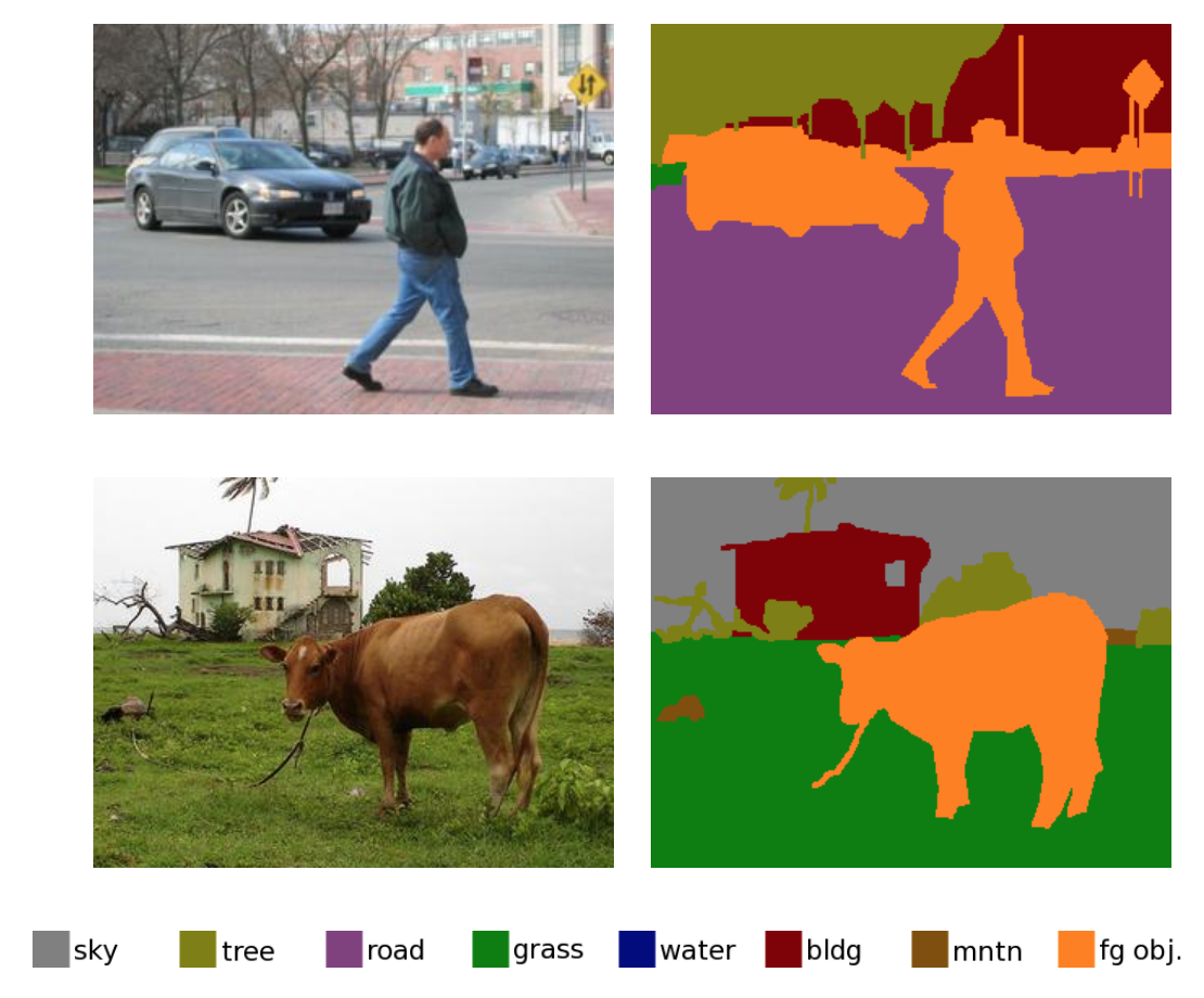
Semantic segmentation is a computer vision task in which we classify the different parts of a visual input into semantically interpretable classes. By “semantically interpretable,” we mean that the classes have some real-world meaning. For instance, we might want to take all the pixels of an image that belong to cars and color them blue.
While unsupervised methods such as clustering can be used for segmentation, the results are not necessarily semantic. These methods do not segment classes they have been trained on, but instead find region boundaries more generally — see Thoma et al. 2016[1].
Semantic segmentation lets us achieve a much more detailed understanding of imagery than image classification or object detection. This detailed understanding is critical in a broad range of fields, including autonomous driving, robotics, and image search engines[2]. In this article, we focus specifically on supervised semantic segmentation using deep learning methods.
Datasets and metrics
Some datasets that are often used for training semantic segmentation models include:
- Pascal VOC 2012: Focuses on 20 object classes, in categories such as Person, Vehicle, and others. Goal is to segment the object class or background.
- Cityscapes: Dataset of semantic urban scene understanding from 50 cities.
- Pascal Context: Indoor and outdoor scenes with 400+ classes.
- Stanford Background Dataset: A set of outdoor scenes with at least one foreground object.
A standard metric that is used to evaluate the performance of semantic segmentation algorithms is Mean IoU (Intersection Over Union), where IoU is defined as:
$$\text{IOU} = \frac{\text{Area of Overlap}}{\text{Area of Union}} = \frac{A_{pred} \cap A_{true}}{A_{pred} \cup A_{true}}$$
Such a metric ensures we capture each object (making predicted labels overlap with the ground truth), but also do so precisely (making union as close as possible to overlap).
Pipeline
At a high level, often, the pipeline for applying models for semantic segmentation is as follows:
$$\text{Input} \rightarrow \text{Classifier} \rightarrow \text{Post-Processing} \rightarrow \text{Final Result}$$
We will further discuss both the Classifier and Post-Processing phase of this pipeline in the following sections.
Architectures and methods
Classification with convolutional neural networks
Recent architectures for semantic segmentation most commonly use convolutional neural networks (CNNs) to assign an initial class label for each pixel. Convolutional layers can effectively capture local features in images, and by nesting many such layers in a hierarchical manner, CNNs attempt to extract broader structure. Through successive convolutional layers that capture increasingly complex features in the image, a CNN can encode an image as a compact representation of its contents.
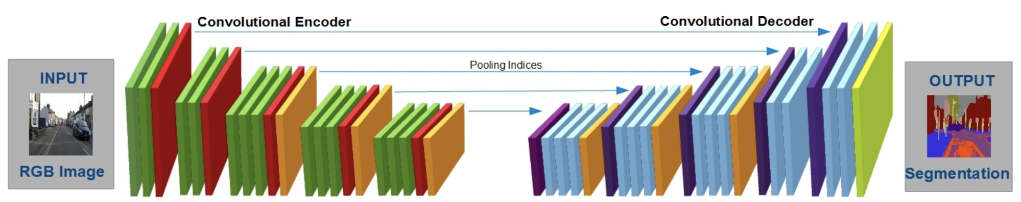
But to map individual pixels to labels, we need to augment the standard CNN encoder into an encoder-decoder setup. In this setup, the encoder uses convolution and pooling layers to reduce the image to a lower-dimensional representation by width and height. The decoder takes that representation and “restores” the spatial dimensions by upsampling (through transpose convolutions), expanding the size of the representation at each decoder step. In some cases, the intermediate steps in the encoder step are used to aid each decoder step. Eventually, the decoder generates an array denoting the labeling of the original image.
In many semantic segmentation architectures, the loss function that the CNN aims to minimize is cross-entropy loss. This objective function measures the distance between each pixel’s predicted probability distribution (over the classes) and its actual probability distribution.
However, cross-entropy loss isn’t ideal for semantic segmentation. Since the final loss for an image is simply the sum of the losses for each pixel, cross-entropy loss doesn’t encourage nearby pixels to be consistent. Because cross-entropy loss fails to impose higher-level structure between the pixels, a labeling that minimizes cross-entropy loss often turns out to be patchy or fuzzy, and will require post-processing.
Refinement with Conditional Random Fields
The raw labeling from the CNN is often a “patchy” image, in which small areas may have incorrect labels that do not match their surrounding pixels’ labels. To fix this discontinuity, we can apply a form of smoothing. We would like to ensure objects occupy connected regions in the image, and that a given pixel likely has the same label as most of its neighbors.
To address this, some architectures use conditional random fields (CRFs)[3] that use the pixel similarities within the original image to refine the CNN’s labeling.
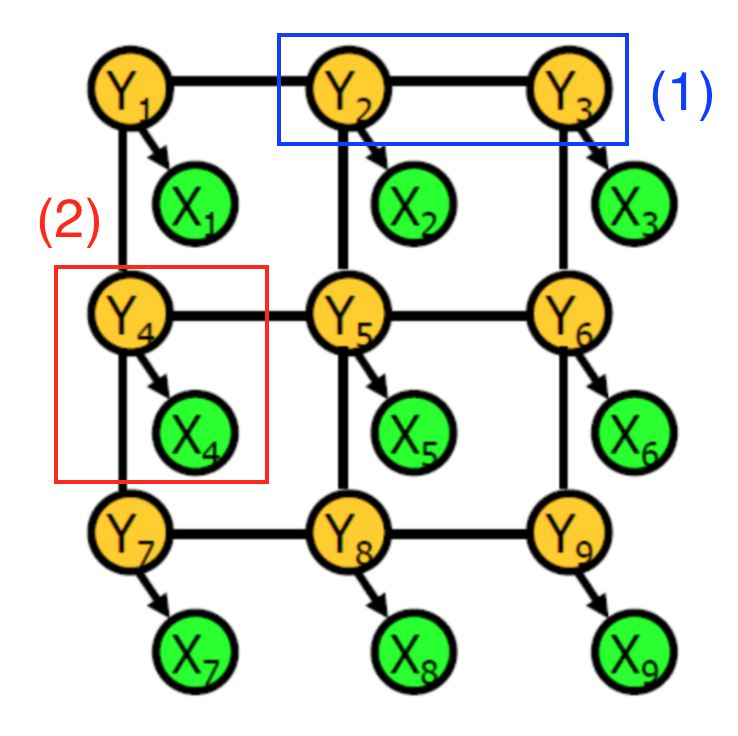
A conditional random field is a graph of random variables. In this context, each vertex represents either
- The CNN’s label of a certain pixel (Green vertices $X_i$)
- The actual object label of a certain pixel (Yellow vertices $Y_i$)
Edges encode two types of information:
- (1) in blue: The dependency between the actual object labels of two pixels physically close to each other
- (2) in red: The dependency between the CNN’s raw prediction and the actual object label for a given pixel
Each dependency is associated with a potential, which is a function on the values of its two associated random variables. For instance, the first type of dependency may have a potential that is high when the actual object labels of the adjacent pixels are the same. Intuitively, the object labels serve as hidden variables, which produce observable CNN pixel labels according to some probability distribution.
To use CRFs to refine a labeling, we first learn the parameters for the graphical model with the training data, via cross-validation. Then, we modify the parameters to maximize the probability $P(Y_1, Y_2, … Y_n | X_1, X_2, … X_n)$. The output of the CRF inference is the final object labeling for the original image’s pixels.
In practice, the CRF graphs are fully connected, meaning that nodes corresponding to pixels physically far apart can still share an edge. Such graphs have billions of edges, making exact inference computationally intractable. CRF architectures tend to use efficient approximation techniques for inference.
Classifier Architectures
CNN classification followed by CRF refinement is just one example of a possible semantic segmentation procedure. Several research papers have described variations on this theme:
-
U-Net (2015)[4] augments its training data by producing distorted versions of the original training data. This step allows the CNN encoder-decoder to be robust against such deformations and to learn from fewer training images. When trained on biomedical datasets with less than 40 images, it stills achieves IOU scores reaching 92%.
-
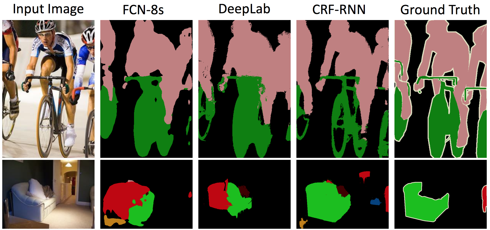
DeepLab (2016)[5] combines a CNN encoder-decoder with CRF refinement to produce its object labels (the authors emphasize the upsampling for the decoding step, as described previously). Atrous convolutions (also called dilated convolutions) use filters of different sizes in each layer, which allows each layer to capture features at a variety of scales. On the Pascal VOC 2012 test set, this architecture achieves a mean IOU of 70.3%.
-
Dilation10 (2016)[6] is an alternate approach applying dilated convolution. The full pipeline attaches the dilated convolution “front-end module” to a context module and a CRF-RNN for further processing. With this configuration, Dilation10 achieves a mean IOU of 75.3%, on the Pascal VOC 2012 test set.
Other Training Schemes
We now turn to recent training schemes that stray from the classifier and CRF model. Rather than consisting of components/ optimized separately, there methods are end-to-end.
Fully Differentiable Conditional Random Fields
The CRF-RNN model by Zheng et al.[7] introduces an approach that combines classification and post-processing into a single end-to-end model, optimizing both phases jointly. Thus, parameters such as the weights of the CRF Gaussian kernels are learned automatically. They achieve this by reformulating a step of the inference approximation algorithm as a convolution, and by using a recurrent neural network (RNN) to model the full iterative nature of the inference algorithm.
Adversarial Training
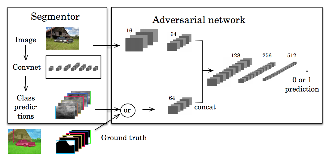
Another recent line of work has focused on using adversarial training to help develop higher-order consistency. Inspired by the generative adversarial networks (GANs), Luc et al. train a standard CNN for semantic segmentation alongside an adversarial network that tries to learn to discriminate between ground-truth segmentations and those predicted by the segmentation network. The segmentation network aims to produce segmentations that the adversarial network cannot distinguish from the true segmentations.
The idea here is that we want our segmentations to seem as real as possible. If some other network can easily separate predictions from the ground truth, then our predictions aren’t good enough.
Segmentation over time
How can we predict where an object will be in the future? We can approach this by modeling the progression of segmentations in a scene. This has applications in robotics or autonomous vehicles, where modeling the motion of objects is useful for planning.
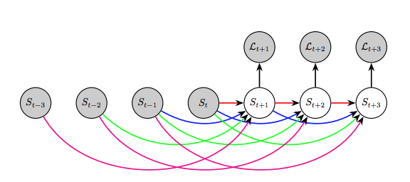
We see this first explored in Luc et al. 2017[8], which demonstrates that directly predicting future semantic segmentations yields higher performance than predicting future frames and then segmenting them.
They use an autoregressive model, where they take past segmentations to predict the next segmentation $S_{t+1}$. For predicting a segmentation $S_{t+2}$ after that, they take the past $S_i$ in combination with the predicted frame $S_{t+1}$, and so on.
They compared their performance on various timescales: predicting the next frame (short-term timescale), predicting the next 0.5 seconds (medium-term timescale), and predicting the next 10 seconds (long-term timescale), evaluating on the Cityscapes dataset. They found poor performance at long timescales, but found good results at short and medium-term timescales. In particular, their approach outperformed a baseline consisting of classical techniques based on optical flow[9].
Final thoughts
Many of these methods, such as U-Net, follow a basic structure: we apply deep learning (convolutional networks), followed by post-processing with classical probabilistic techniques. While the raw outputs of a convolutional network can be imperfect, post-processing better aligns the segmentation with human intuition for a “good” labeling.
The remaining methods, such as adversarial learning, serve as powerful end-to-end solutions for segmentation. End-to-end techniques do not require humans to model individual components to refine raw predictions, unlike the CRF step described previously. As these solutions currently perform better than multistage pipelines, future research might come to focus more and more on end-to-end algorithms.
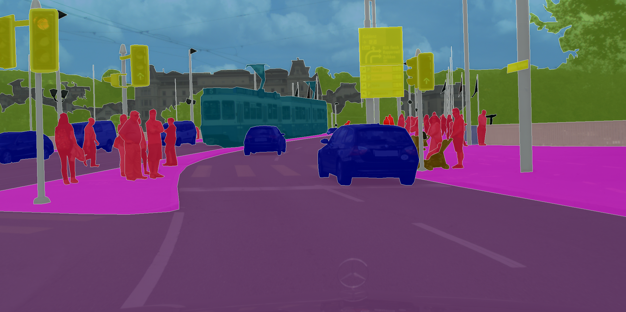
Cover image: a segmentation of a road in Zurich, from the Cityscapes dataset.
Citation
For attribution in academic contexts or books, please cite this work as
Andy Chen and Chaitanya Asawa, "Going beyond the bounding box with semantic segmentation", The Gradient, 2018.
BibTeX citation:
@article{achen2018semanticsegments,
author = {Chen, Andy, Asawa, Chaitanya},
title = {Going beyond the bounding box with semantic segmentation},
journal = {The Gradient},
year = {2018},
howpublished = {\url{https://thegradient.pub/semantic-segmentation/ } },
}
If you enjoyed this piece and want to hear more, subscribe to the Gradient and follow us on Twitter.
Thoma, Martin. "A survey of semantic segmentation." arXiv preprint arXiv:1602.06541 (2016). ↩︎
The literature review by Garcia-Garcia et al. 2017 examines different approaches in detail. ↩︎
Lafferty, John, Andrew McCallum, and Fernando CN Pereira. "Conditional random fields: Probabilistic models for segmenting and labeling sequence data." (2001). ↩︎
Ronneberger, Olaf, Philipp Fischer, and Thomas Brox. "U-net: Convolutional networks for biomedical image segmentation." International Conference on Medical image computing and computer-assisted intervention. Springer, Cham, 2015. ↩︎
Chen, Liang-Chieh, et al. "Deeplab: Semantic image segmentation with deep convolutional nets, atrous convolution, and fully connected crfs." IEEE transactions on pattern analysis and machine intelligence 40.4 (2018): 834-848. ↩︎
Yu, Fisher, and Vladlen Koltun. "Multi-scale context aggregation by dilated convolutions." arXiv preprint arXiv:1511.07122 (2015). ↩︎
Zheng, Shuai, et al. "Conditional random fields as recurrent neural networks." Proceedings of the IEEE International Conference on Computer Vision. 2015. ↩︎
Luc, Pauline, et al. "Semantic segmentation using adversarial networks." arXiv preprint arXiv:1611.08408 (2016). ↩︎
Fortun, Denis, Patrick Bouthemy, and Charles Kervrann. "Optical flow modeling and computation: a survey." Computer Vision and Image Understanding 134 (2015): 1-21. ↩︎
