We have an incredible amount of information about how objects are related. But most of us have no idea how to use it.

Network graphs of interactions and friendships on social media are rich with useful insights. Synonym graphs like WordNet can help us better identify related objects in a scene with computer vision. From family trees to molecular structures, an enormous amount of information around us takes the form of graphs.

But despite its prevalence, graph structure is often discarded when applying machine learning. Consider the fashion recommendation problem, whose goal is to find sets of clothing items that constitute a cohesive, possibly personalized “style.” A common approach is to scrape images from social media, identify the clothing in these images, and then use the images’ popularity as a proxy for how “fashionable” a basket of clothing is. While it’s possible to learn fashion styles this way, this model could easily be improved with graph data; we can analyze fashion trends in the user's social network, for instance, or extract clusters in the Amazon related-product graph.

So why is structural information often ignored? The answer, for the most part, is that it’s notoriously challenging to extract meaningful features from graphs.

In this article, we will explore recent techniques that aim to extract meaningful features from graphs. In particular, we'll focus on methods that harness random walks to quantify similarity between nodes in a graph. These techniques predominantly draw upon existing results by the natural language processing community. I'll suggest a few future avenues of research relating, in particular, to learning features over time-varying graphs. Finally, we'll briefly discuss the family of graph convolutional networks (GCNs), which provide an end-to-end solution to machine learning over structured data that does not require an intermediate feature extraction step.

These methods constitute a subfield of machine learning in themselves, but ML researchers and practitioners across the board can benefit from exploiting structure in their specific domains of interest.

$\newcommand{\argmin}{\text{arg min}}\newcommand{\argmax}{\text{arg max}}\newcommand{\minimize}{\text{minimize}}\newcommand{\maximize}{\text{maximize}}\newcommand{\abs}{\text{abs}}\newcommand{\mbf}{\mathbf}$

Learning features on graphs

Summarizing graphs

When doing machine learning on graphs, it’s often useful to compute a graph summary, which maps each vertex to a real-valued feature vector that encodes its neighborhood. We want to learn a function that maps two vertices to similar feature vectors in $\mathbb{R}^d$ if they have similar neighborhoods. (The term “neighborhood” is broad, but it typically aims to capture some notion of locality, such as the set of vertices 1 or 2 hops away from a vertex.)

The feature vectors of each vertex in the graph can then be stacked into a matrix $F \in \mathbb{R}^{|V| \times d}$ of latent features. This is a nice, vectorized representation that we can then run standard machine learning algorithms on.

DeepWalk (2014) and node2vec (2016) are two algorithms for learning these feature vectors. Let’s find out how these work.

DeepWalk: random walks as sentences?

The key insight behind the DeepWalk algorithm is that random walks in graphs are a lot like sentences. It’s been experimentally observed that both words in a sentence and random walks on a real-world graph follow a power-law distribution, which means that we can imagine these random walks as “sentences” in a certain “language.”

Motivated by this similarity, DeepWalk builds graph summaries through optimization techniques originally developed for natural language modelling. In standard language modeling, we learn to estimate the probability that a word appears in a sentence, given the words around it. DeepWalk, on the other hand, learns to estimate the probability that a vertex appears in a random walk, given the vertices before it. And, like in a language model, we‘re trying to learn feature vectors $\mathbf{f}^{u_i}$ of the vertices $u_i$ that help us estimate this probability. To put it concretely, given some classifier that estimates $\Pr[u_i~|~(\mathbf{f}^{u_1},\ldots,\mathbf{f}^{u_{i-1}})]$, our goal is choose feature vectors $F \in \mathbb{R}^{n \times d}$ that maximize

\begin{equation}
\Pr[u_i~|~(\mathbf{f}^{u_1},\ldots,\mathbf{f}^{u_{i-1}})].
\end{equation}

However, this objective is intractable as the length of the random walk grows. Thus, the authors instead reframe the problem in terms of predicting the nearest $2w$ neighbors of a vertex $u_i$ given its representation $\mathbf{f}^{u_i}$. (This is technically a different optimization problem, but it serves as a reasonable, order-independent alternative to the previous objective.) In other words, we want to maximize the probability

\begin{equation} \Pr[u_{i - w},\ldots,u_{i-1},u_{i+1},\ldots,u_{i + w}~|~\mathbf{f}^{u_i}]. \end{equation}

But how do we minimize this objective over the space of all random walks? One strategy is this¹:

• Sample a vertex $v$ and generate a random walk $v_1, \ldots, v_t$, where $v_1 = v$.
• For each $v_j$ in the walk, and for each $u_k$ less than a certain number of steps away, apply gradient descent on $\mathbf{F}$ to minimize the loss $J(\mathbf{F}) = -\log \Pr u_k | F_{v_j}$.

This algorithm works, but its description masks the complexity of the final gradient descent step, which requires small updates to at least $|\mathbf{V}| \times d$ parameters. This is a serious problem if the graph’s size is in the millions.

To address this, the authors approximate the conditional probability using “hierarchical softmax,” which, while outside of the scope of this article, breaks the optimization into a balanced tree of binary classifiers. Using these binary classifiers, they reduce the number of parameters that need to be updated in a single gradient descent step from $O(|\mathbf{V}|\times d)$ to $O(\log|\mathbf{V}| \times d)$.

Node2vec: generalizing to different types of neighborhoods

Grover and Leskovec (2016) generalize DeepWalk into the node2vec algorithm. Instead of “first-order” random walks that choose the next node based only on the current node, node2vec uses a family of “second-order” random walks that depend on both the current node and the one before it.

We can specify the exact distribution at each step through the parameters $p, q \in \mathbb{R}$: roughly speaking, we can bias the walks towards “exploration” by lowering $p$, and toward “breadth-first” behavior by raising $q$. The key insight of the paper is that we can draw attention to different properties of the graph by choosing different kinds of second-order random walks.

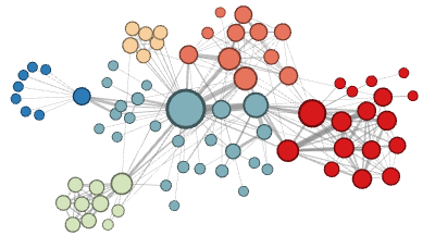
To show why this is necessary, the authors identify two general types of neighborhoods of neighborhoods for machine learning on graphs (photos from Grover and Lesokovec

• Under the homophily hypothesis, highly connected nodes are part of the same neighborhood since they are proximate to each other in the graph.
  

• Under the structural hypothesis, nodes that serve similar structural functions — for example, nodes that act as a hub — are part of the same neighborhood due to their higher-order structural significance.
  

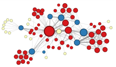
Using two tuning parameters $p, q \in \mathbb{R}$, the authors provide a smooth way to interpolate between these two conceptions of neighborhoods.

Just as with DeepWalk, the node2vec objective can be optimized by sampling $v_i \in \mathbf{V}$, taking a $(p, q)$ random walk $v_1, \dots, v_t$ where $v_1 = v_i$ and updating $\mbf{F}$ through gradient descent.

Latent features over temporal networks

These graph summarization techniques are useful, but many real-world graphs are temporal networks—that is, they change over time. For instance, a user’s graph of friends on a social network can grow and shrink over time. We could apply node2vec, but there are two downsides.

• It could be computationally expensive to run a new instance of node2vec every time the graph is modified.
• Additionally, there is no guarantee that multiple applications of node2vec will produce similar or even comparable matrices $\mbf{F}$.

Here’s a strategy to resolve the first problem — instead of reapplying node2vec after each modification, we can wait until enough edges have been modified to lower the quality of the original embedding $\mbf{F}$.

But how many edges constitute a “significant” enough change? This depends highly on the specific edges in the graph and the $(p, q)$-character of the random walk. Look at these pairs of graphs:

We might note that the neighborhoods in $K_6-e$ are very similar to those of $K_6$. However, the additional edge that transforms the path graph, $P_6$ into a cycle, $C_6$, significantly changes the random walk neighborhoods of the graph. Edges that act as “bridges” between otherwise disconnected or weakly connected parts of a network will tend to have an outsized impact on neighborhoods.

Luckily, many real-world graphs, like social networks, tend to be more like $K_6-e$. They are often highly connected, to the point where adding or deleting an edge will not affect embeddings significantly for the first-order random walks that DeepWalk uses. But it is important to note that first-order random walks are quite different from second-order ones, so this discussion may not necessarily extend to node2vec.

The second issue can, to some degree, be resolved by concatenating the feature vectors derived for each node from multiple applications of node2vec and then training an autoencoder to map these stacked features into a compressed representation.

How can we achieve scalable feature learning on temporal graphs? For temporal graphs, tools like the dynamic spectral sparsifier by Abraham et al. (2016) might be applied towards incremental updates of graph embeddings. Still, there is significant work to be done. The best sparsifiers are impractically slow on the scale of real-world graphs – while sub-logarithmic algorithms exist, the constant factor of these algorithms can be enormous. I believe that combining ideas of dynamic graph partitioning and updates to the graph summary matrix $\mbf{F}$ may result in a tractable approach to temporal graph feature summarization.

An alternative approach could be to generalize the node2vec algorithm to temporal networks by introducing an additional parameter $\lambda$ that influences the likelihood of random walks to traverse “temporal boundaries.” Some prediction tasks might have a notion of “temporal locality,” in which snapshots of the graph with similar timestamps are related, while others might have longer term dependences.

We will now turn to graph convolutional networks, a more recent approach to perform machine learning on graphs.

A Taste of Graph Convolutional Networks

Node2vec and DeepWalk produce summaries that are later analyzed with a machine learning technique. By contrast, graph convolutional networks (GCNs) present an end-to-end approach to structured learning.

GCN methods seek to generalize traditional convolutional networks to the variable, unordered structures. Since graphs do not have a well-defined order, GCNs must be agnostic to a permutation of the relative ordering of nodes. Clearly, CNNs do not have this property right out of the box, since applying a random permutation matrix to an image before passing it through a CNN is bound to change the output of the computation (often, CNNs for vision problems identify edges or other local structures in images that are not invariant under a permutation of rows and columns of the input). Furthermore, CNNs are not agnostic to the shape of pixel neighborhoods -- there is no obvious way to train a CNN that accepts both images defined over a square and a hexagonal mesh, which have internal pixels with eight and six immediate neighbors, respectively. Consequently, sensible relaxations must be made to the CNN activation function in order to account for the dynamic structure of general graphs.

Various authors have proposed different GCN relaxations. One proposal^[1] defines an analogue to CNNs that optimizes over sparse filters that operate on clusterings of the graph at multiple scales. The paper also gives a spectral analogue to CNNs in which multiple spectral filters operate on the eigenvectors corresponding to the largest eigenvalues. Another proposal ^[2] presents a scheme for GCN updates with the same time complexity as CNN updates by considering only low-degree polynomial approximation of the spectral filters. A third proposal^[3] simplifies the GCN formulation by layering multiple linear spectral filters that can together capture higher order features.

These graph convolutional network formulations are interesting in their own right and require more space to characterize in detail. Yet, GCNs already show promise as a reasonable alternative to the graph summarization methods described in the previous section. GCNs also benefit from their entirely differentiable characterizations, which permit the sparse filters to be tuned as part of an end-to-end learning algorithm. Even though the bias hyper-parameters of node2vec permit more personalized features to be discovered, GCN weight matrices are tuned based on the provided training data.

Structured learning has already been applied to biochemical research: one paper^[4] provides an end-to-end and fully-differentiable neural network for predicting protein-ligand affinity that harnesses sparse atomic structure. Another paper^[5], tackles drug discovery with GCNs and introduces a dummy “super node” connected by a directed edge to every node in the graph representation of the candidate drug in order to derive graph-level features. GCNs have also been successfully employed in link prediction and entity classification over knowledge graphs^[6]. The recent success of structured learning and the brisk pace of research suggest that much more is to come in the next few years. Perhaps we'll soon see GCN networks that leverage relational structure such as knowledge graphs to improve the performance of object detection in computer vision. Or perhaps protein-folding simulation will soon be accelerated by structured learning methods that drastically reduce the dimensionality of three-dimensional proteins with low atomic degree. These applications are almost certainly on the horizon (if not already en route to publication!), which certainly makes structured learning an exciting field to follow.

---

Citation
For attribution in academic contexts or books, please cite this work as

Matthew Das Sarma, "How do we capture structure in relational data?", The Gradient, 2018.

BibTeX citation:

@article{msarma2018structureleanring,
author = {Sarma, Matthew Das},
title = {How do we capture structure in relational data?},
journal = {The Gradient},
year = {2018},
howpublished = {\url{https://thegradient.pub/structure-learning/ } },
}

---

If you enjoyed this piece and want to hear more, subscribe to the Gradient and follow us on Twitter.

---

1. Bruna, Joan, et al. "Spectral networks and locally connected networks on graphs." arXiv preprint arXiv:1312.6203 (2013). ↩︎

2. Defferrard, Michaël, Xavier Bresson, and Pierre Vandergheynst. "Convolutional neural networks on graphs with fast localized spectral filtering." Advances in Neural Information Processing Systems. 2016. ↩︎

3. Kipf, Thomas N., and Max Welling. "Semi-supervised classification with graph convolutional networks." arXiv preprint arXiv:1609.02907 (2016). ↩︎

4. Gomes, Joseph, et al. "Atomic convolutional networks for predicting protein-ligand binding affinity." arXiv preprint arXiv:1703.10603 (2017). ↩︎

5. Li, Junying, Deng Cai, and Xiaofei He. "Learning Graph-Level Representation for Drug Discovery." arXiv preprint arXiv:1709.03741 (2017). ↩︎

6. Schlichtkrull, Michael, et al. "Modeling Relational Data with Graph Convolutional Networks." arXiv preprint arXiv:1703.06103 (2017). ↩︎