Geometric Deep Learning is an umbrella term for approaches considering a broad class of ML problems from the perspectives of symmetry and invariance. It provides a common blueprint allowing to derive from first principles neural network architectures as diverse as CNNs, GNNs, and Transformers. Here, we study how these ideas have emerged through history from ancient Greek geometry to Graph Neural Networks.

The last decade has witnessed an experimental revolution in data science and machine learning, epitomised by deep learning methods. Indeed, many high-dimensional learning tasks previously thought to be beyond reach — computer vision, playing Go, or protein folding — are in fact feasible with appropriate computational scale. Remarkably, the essence of deep learning is built from two simple algorithmic principles: first, the notion of representation or feature learning, whereby adapted, often hierarchical, features capture the appropriate notion of regularity for each task, and second, learning by gradient descent-type optimisation, typically implemented as backpropagation.

While learning generic functions in high dimensions is a cursed estimation problem, most tasks of interest are not generic and come with essential predefined regularities arising from the underlying low-dimensionality and structure of the physical world. Geometric Deep Learning is concerned with exposing these regularities through unified geometric principles that can be applied throughout a broad spectrum of applications.

Exploiting the known symmetries of a large system is a powerful and classical remedy against the curse of dimensionality, and forms the basis of most physical theories. Deep learning systems are no exception, and since the early days, researchers have adapted neural networks to exploit the low-dimensional geometry arising from physical measurements, e.g. grids in images, sequences in time-series, or position and momentum in molecules, and their associated symmetries, such as translation or rotation.

Since these ideas have deep roots in science, we will attempt to see how they have evolved throughout history, culminating in a common blueprint that can be applied to most of today’s popular neural network architectures.

Order, Beauty, and Perfection

“Symmetry, as wide or as narrow as you may define its meaning, is one idea by which man through the ages has tried to comprehend and create order, beauty, and perfection.” — Hermann Weyl (1952)

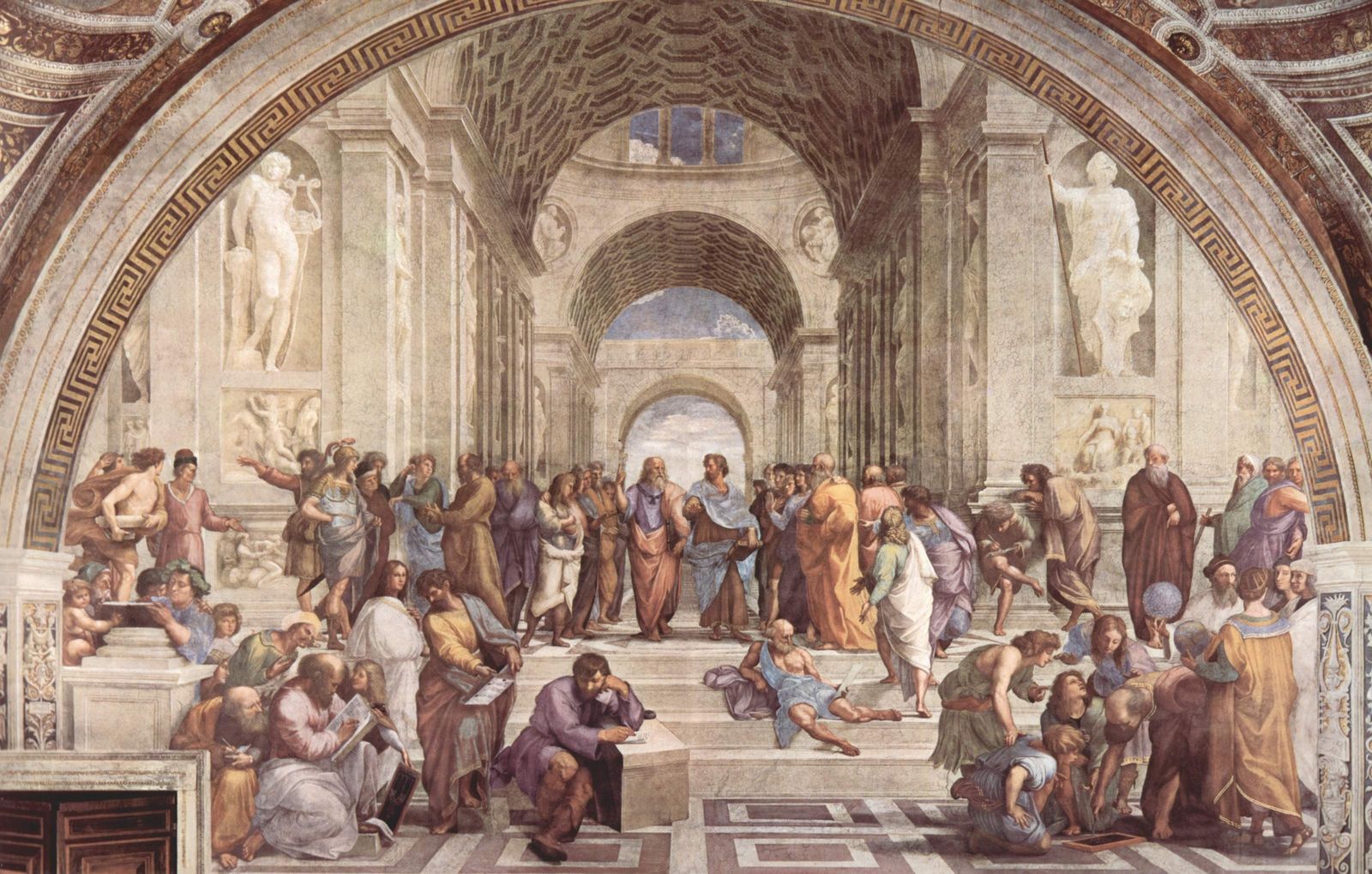
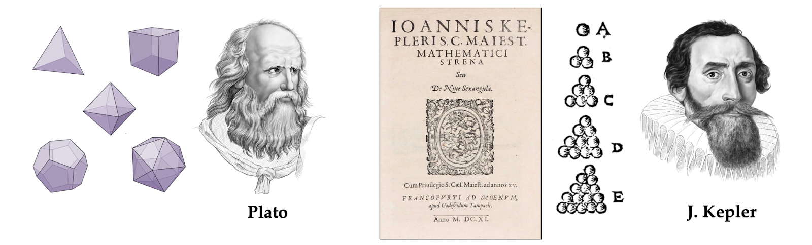
This somewhat poetic definition of symmetry is given in the eponymous book of the great mathematician Hermann Weyl [1], his Schwanengesang on the eve of retirement from the Institute for Advanced Study in Princeton. Weyl traces the special place symmetry has occupied in science and art to ancient times, from Sumerian symmetric designs to the Pythagoreans, who believed the circle to be perfect due to its rotational symmetry. Plato considered the five regular polyhedra bearing his name today so fundamental that they must be the basic building blocks shaping the material world.

Yet, though Plato is credited with coining the term συμμετρία (‘symmetria’) which literally translates as ‘same measure’, he used it only vaguely to convey the beauty of proportion in art and harmony in music. It was the German astronomer and mathematician Johannes Kepler who attempted the first rigorous analysis of the symmetric shape of water crystals. In his treatise ‘On the Six-Cornered Snowflake’ [2], he attributed the six-fold dihedral structure of snowflakes to hexagonal packing of particles — an idea that though preceded the clear understanding of how matter is formed, still holds today as the basis of crystallography [3].

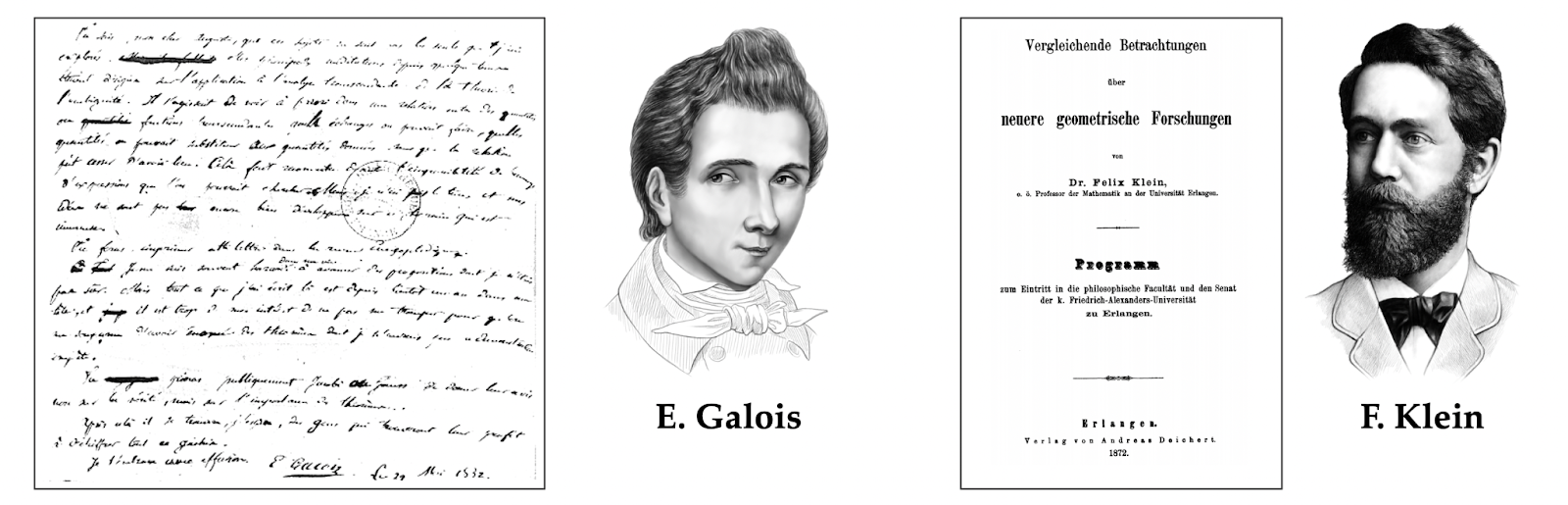
In modern mathematics, symmetry is almost univocally expressed in the language of group theory. The origins of this theory are usually attributed to Évariste Galois, who coined the term and used it to study the solvability of polynomial equations in the 1830s [4]. Two other names associated with group theory are those of Sophus Lie and Felix Klein, who met and worked fruitfully together for a period of time [5]. The former would develop the theory of continuous symmetries that today bears his name (Lie groups); the latter proclaimed group theory to be the organising principle of geometry in his Erlangen Programme. Given that Klein’s Programme is the inspiration for Geometric Deep Learning, it is worthwhile to spend more time on its historical context and revolutionary impact.

A Strange New World

The foundations of modern geometry were formalised in ancient Greece nearly 2300 years ago by Euclid in a treatise named the Elements. Euclidean geometry (which is still taught at school as ‘the geometry’) was a set of results built upon five intuitive axioms or postulates. The Fifth Postulate — stating that it is possible to pass only one line parallel to a given line through a point outside it — appeared less obvious and an illustrious row of mathematicians broke their teeth trying to prove it since antiquity, to no avail.

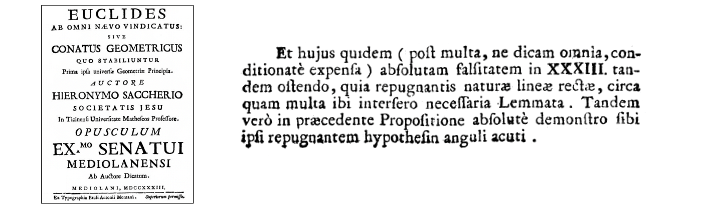
An early approach to the problem of the parallels appears in the eleventh-century Persian treatise ‘A commentary on the difficulties concerning the postulates of Euclid’s Elements’ by Omar Khayyam [6]. The eighteenth-century Italian Jesuit priest Giovanni Saccheri was likely aware of this previous work judging by the title of his own work Euclides ab omni nævo vindicatus (‘Euclid cleared of every stain’).

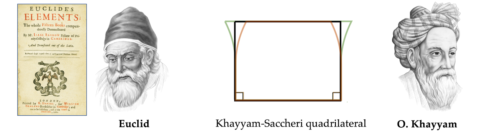
Like Khayyam, he considered the summit angles of a quadrilateral with sides perpendicular to the base. The conclusion that acute angles lead to infinitely many non-intersecting lines that can be passed through a point not on a straight line seemed so counter-intuitive that he rejected it as ‘repugnatis naturæ linæ rectæ’ (‘repugnant to the nature of straight lines’) [7].

The nineteenth century has brought the realisation that the Fifth Postulate is not essential and one can construct alternative geometries based on different notions of parallelism. One such early example is projective geometry, arising, as the name suggests, in perspective drawing and architecture. In this geometry, points and lines are interchangeable, and there are no parallel lines in the usual sense: any lines meet in a ‘point at infinity.’ While results in projective geometry had been known since antiquity, it was first systematically studied by Jean-Victor Poncelet in 1812 [8].

The credit for the first construction of a true non-Euclidean geometry is disputed. The princeps mathematicorum Carl Friedrich Gauss worked on it around 1813 but never published any results [9]. The first publication on the subject of non-Euclidean geometry was ‘On the Origins of Geometry’ by the Russian mathematician Nikolai Lobachevsky [10]. In this work, he considered the Fifth Postulate an arbitrary limitation and proposed an alternative one, that more than one line can pass through a point that is parallel to a given one. Such construction requires a space with negative curvature — what we now call a hyperbolic space — a notion that was still not fully mastered at that time [11].

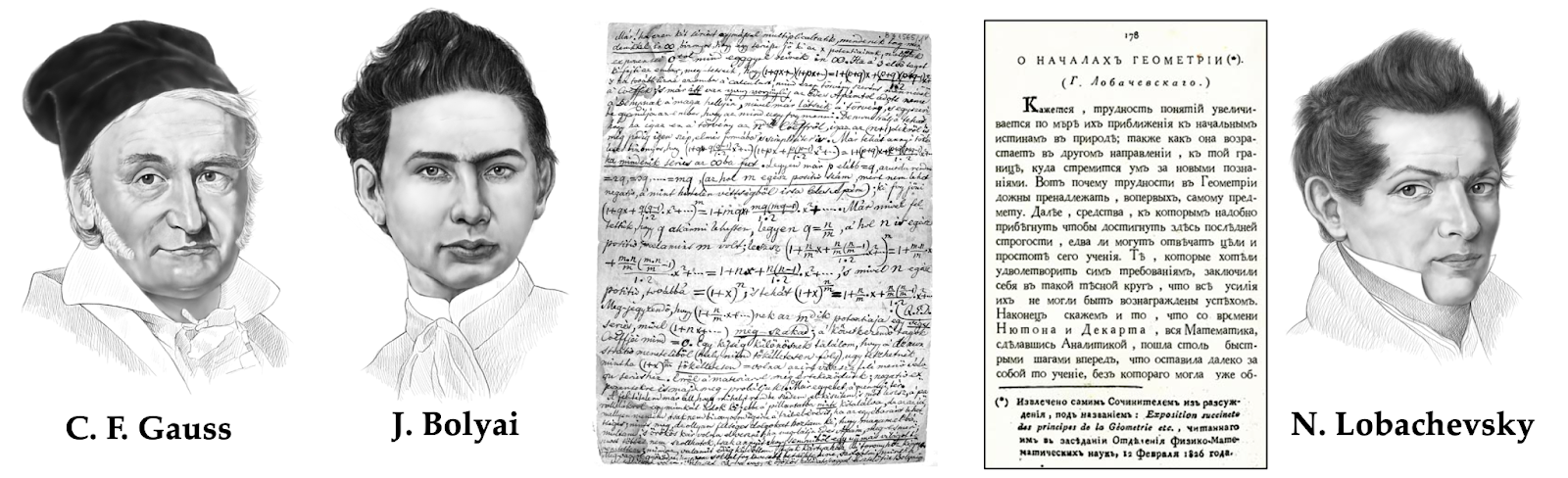
Lobachevsky’s idea appeared heretical and he was openly derided by colleagues [12]. A similar construction was independently discovered by the Hungarian János Bolyai, who published it in 1832 under the name ‘absolute geometry.’ In an earlier letter to his father dated 1823, he wrote enthusiastically about this new development:

“I have discovered such wonderful things that I was amazed… out of nothing I have created a strange new world.” — János Bolyai (1823)

In the meantime, new geometries continued to come out like from a cornucopia. August Möbius [13], of the eponymous surface fame, studied affine geometry. Gauss’ student Bernhardt Riemann introduced a very broad class of geometries — called today Riemannian is his honour — in his habilitation lecture, subsequently published under the title Über die Hypothesen, welche der Geometrie zu Grunde liegen (‘On the Hypotheses on which Geometry is Based’) [14]. A special case of Riemannian geometry is the ‘elliptic’ geometry of the sphere, another construction violating Euclid’s Fifth Postulate, as there is no point on the sphere through which a line can be drawn that never intersects a given line.

Towards the second half of the nineteenth century, Euclid’s monopoly over geometry was completely shattered. New types of geometry (affine, projective, hyperbolic, spherical) emerged and became independent fields of study. However, the relationships of these geometries and their hierarchy were not understood.

It was in this exciting but messy situation that Felix Klein came forth, with a genius insight to use group theory as an algebraic abstraction of symmetry to organise the ‘geometric zoo.’ Only 23 years old at the time of his appointment as a professor in Erlangen, Klein, as it was customary in German universities, was requested to deliver an inaugural research programme — titled Vergleichende Betrachtungen über neuere geometrische Forschungen (‘A comparative review of recent researches in geometry’), it has entered the annals of mathematics as the “Erlangen Programme” [15].

The breakthrough insight of Klein was to approach the definition of geometry as the study of invariants, or in other words, structures that are preserved under a certain type of transformations (symmetries). Klein used the formalism of group theory to define such transformations and use the hierarchy of groups and their subgroups in order to classify different geometries arising from them.

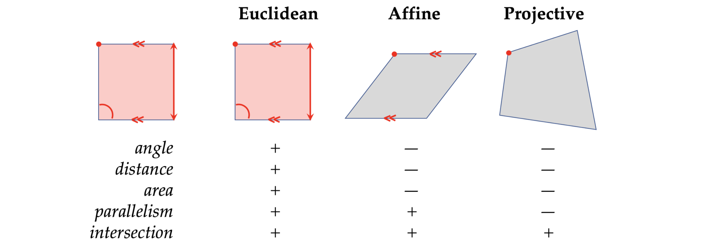
It appeared that Euclidean geometry is a special case of affine geometry, which is in turn a special case of projective geometry (or, in terms of group theory, the Euclidean group is a subgroup of the projective group). Klein’s Erlangen Programme was in a sense the ‘second algebraisation’ of geometry (the first one being the analytic geometry of René Descartes and the method of coordinates bearing his Latinised name Cartesius) that allowed to produce results impossible by previous methods.

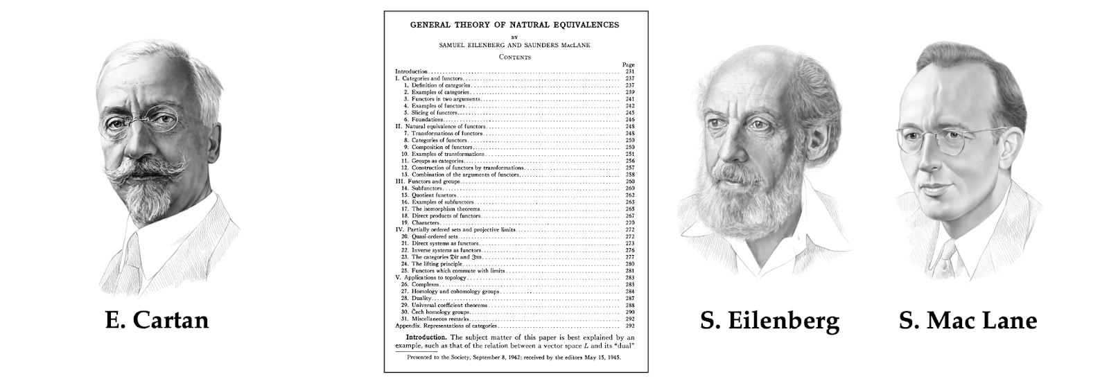
More general Riemannian geometry was explicitly excluded from Klein’s unified geometric picture, and it took another fifty years before it was integrated, largely thanks to the work of Élie Cartan in the 1920s. Furthermore, Category Theory, now pervasive in pure mathematics, can be “regarded as a continuation of the Klein Erlangen Programme, in the sense that a geometrical space with its group of transformations is generalized to a category with its algebra of mappings”, in the words of its creators Samuel Eilenberg and Saunders Mac Lane [16].

The Theory of Everything

Considering projective geometry the most general of all, Klein complained in his Vergleichende Betrachtungen [17]:

“How persistently the mathematical physicist disregards the advantages afforded him in many cases by only a moderate cultivation of the projective view.” — Felix Klein (1872)

His advocating for the exploitation of symmetry in physics has foretold the following century revolutionary advancements in the field.

In Göttingen [18], Klein’s colleague Emmy Noether [19] proved that every differentiable symmetry of the action of a physical system has a corresponding conservation law [20]. It was a stunning result: beforehand, meticulous experimental observation was required to discover fundamental laws such as the conservation of energy. Noether’s Theorem — “a guiding star to 20th and 21st century physics,” in the words of the Nobel laureate Frank Wilczek — allowed for example to show that the conservation of energy emerges from the translational symmetry of time.

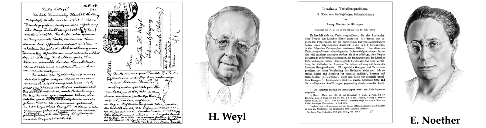
Another symmetry was associated with charge conservation, the global gauge invariance of the electromagnetic field, first appeared in Maxwell’s formulation of electrodynamics [21]; however, its importance initially remained unnoticed. The same Hermann Weyl, who wrote so dithyrambically about symmetry, first introduced the concept of gauge invariance in physics in the early 20th century [22], emphasizing its role as a principle from which electromagnetism can be derived. It took several decades until this fundamental principle — in its generalised form developed by Yang and Mills [23] — proved successful in providing a unified framework to describe the quantum-mechanical behaviour of electromagnetism and the weak and strong forces. In the 1970s, it culminated in the Standard Model that captures all the fundamental forces of nature but gravity [24]. As succinctly put by another Nobel-winning physicist, Philip Anderson [25],

“it is only slightly overstating the case to say that physics is the study of symmetry” — Philip Anderson (1972)

An impatient reader might wonder at this point, what does all this excursion into the history of geometry and physics, however exciting it might be, have to do with deep learning? As we will see, the geometric notions of symmetry and invariance have been recognised as crucial even in early attempts to do ‘pattern recognition,’ and it is fair to say that geometry has accompanied the nascent field of artificial intelligence from its very beginning.

The Rise and Fall of the Perceptrons

While it is hard to agree on a specific point in time when ‘artificial intelligence’ was born as a scientific field (in the end, humans have been obsessed with comprehending intelligence and learning from the dawn of civilisation), we will try a less risky task of looking at the precursors of deep learning — the main topic of our discussion. This history can be packed into less than a century [26].

By the 1930s, it has become clear that the mind resides in the brain, and research efforts turned to explaining brain functions such as memory, perception, and reasoning, in terms of brain network structures. McCulloch and Pitts [27] are credited with the first mathematical abstraction of the neuron, showing its capability to compute logical functions. Just a year after the legendary Dartmouth College workshop that coined the very term ‘artificial intelligence’ [28], an American psychologist Frank Rosenblatt from Cornell Aeronautical laboratory proposed a class of neural networks he called ‘perceptrons’ [29].

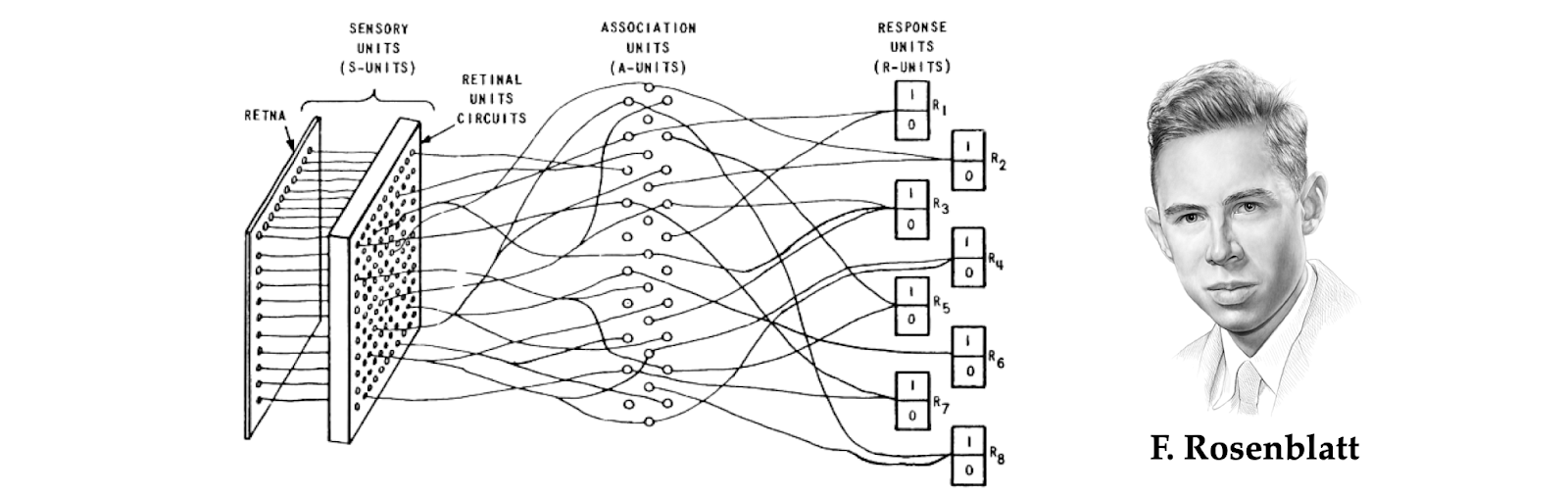
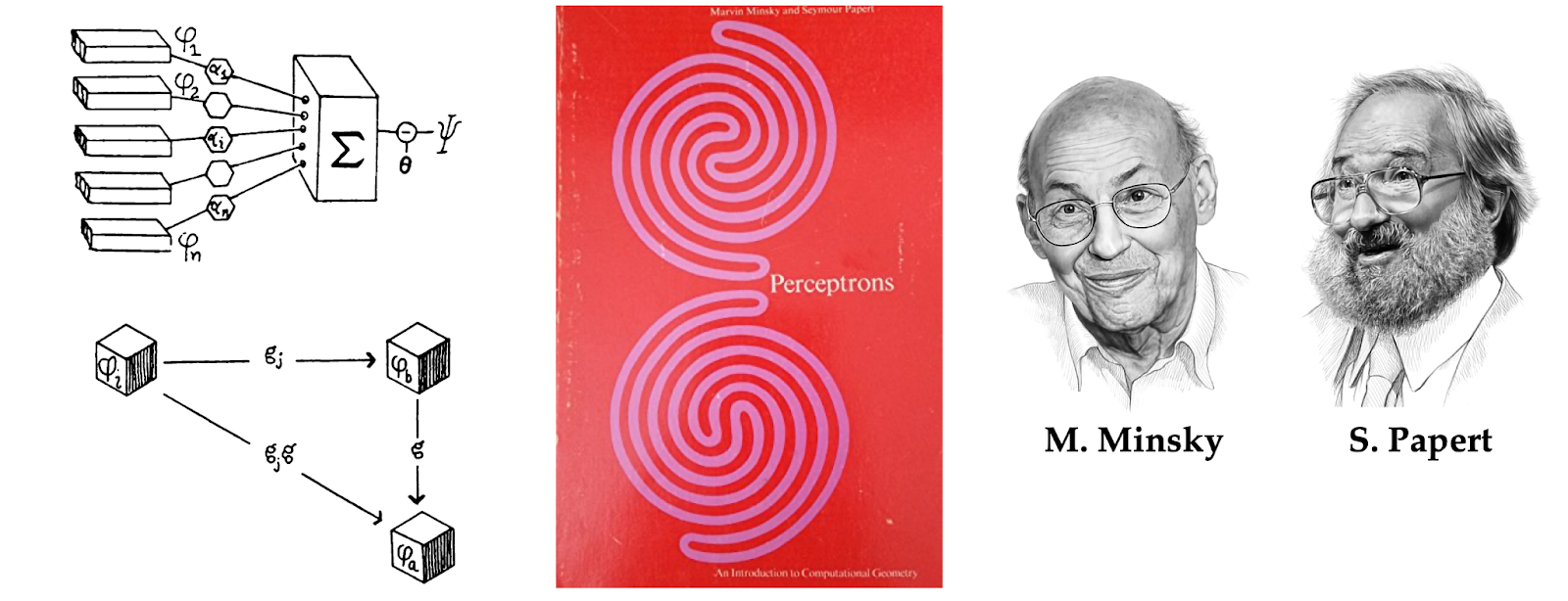
Perceptrons, first implemented on a digital machine and then in dedicated hardware, managed to solve simple pattern recognition problems such as classification of geometric shapes. However, the quick rise of ‘connectionism’ (how AI researchers working on artificial neural networks labeled themselves) received a bucket of cold water in the form of the now-infamous book Perceptrons by Marvin Minsky and Seymour Papert [30].

In the deep learning community, it is common to retrospectively blame Minsky and Papert for the onset of the first ‘AI Winter,’ which made neural networks fall out of fashion for over a decade. A typical narrative mentions the ‘XOR Affair,’ a proof that perceptrons were unable to learn even very simple logical functions as evidence of their poor expressive power. Some sources even add a pinch of drama recalling that Rosenblatt and Minsky went to the same school and even alleging that Rosenblatt’s premature death in a boating accident in 1971 was a suicide in the aftermath of the criticism of his work by colleagues.

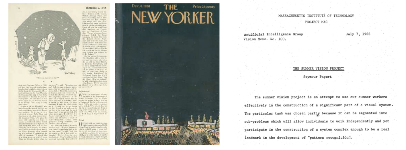
The reality is probably more mundane and more nuanced at the same time. First, a far more plausible reason for the ‘AI Winter’ in the USA is the 1969 Mansfield Amendment, which required the military to fund “mission-oriented direct research, rather than basic undirected research.” Since many efforts in artificial intelligence at the time, including Rosenblatt’s research, were funded by military agencies and did not show immediate utility, the cut in funding has had dramatic effects. Second, neural networks and artificial intelligence in general were over-hyped: it is enough to recall a 1958 New Yorker article calling perceptrons a

“first serious rival to the human brain ever devised” — The New Yorker (1958)

and “remarkable machines” that were “capable of what amounts to thought” [31], or the overconfident MIT Summer Vision Project expecting a “construction of a significant part of a visual system” and achieving the ability to perform “pattern recognition” [32] during one summer term of 1966. A realisation by the research community that initial hopes to ‘solve intelligence’ had been overly optimistic was just a matter of time.

If one, however, looks into the substance of the dispute, it is apparent that what Rosenblatt called a ‘perceptron’ is rather different from what Minsky and Papert understood under this term. Minsky and Papert focused their analysis and criticism on a narrow class of single-layer neural networks they called ‘simple perceptrons’ (and what is typically associated with this term in modern times) that compute a weighted linear combination of the inputs followed by a nonlinear function [33]. On the other hand, Rosenblatt considered a broader class of architectures that antedated many ideas of what would now be considered ‘modern’ deep learning, including multi-layered networks with random and local connectivity [34].

Rosenblatt could have probably rebutted some of the criticism concerning the expressive power of perceptrons had he known about the proof of the Thirteenth Hilbert Problem [35] by Vladimir Arnold and Andrey Kolmogorov [36-37] establishing that a continuous multivariate function can be written as a superposition of continuous functions of a single variable. The Arnold–Kolmogorov theorem was a precursor of a subsequent class of results known as ‘universal approximation theorems’ for multi-layer (or ‘deep’) neural networks that put these concerns to rest.

While most remember the book of Minsky and Papert for the role it played in cutting the wings of the early day connectionists and lament the lost opportunities, an important overlooked aspect is that it for the first time presented a geometric analysis of learning problems. This fact is reflected in the very name of the book, subtitled ‘An introduction to Computational Geometry.’ At the time it was a radically new idea, and one critical review of the book [38] (which essentially stood in the defense of Rosenblatt), questioned:

“Will the new subject of “Computational Geometry” grow into an active field of mathematics; or will it peter out in a miscellany of dead ends?” — Block (1970)

The former happened: computational geometry is now a well-established field [39].

Furthermore, Minsky and Papert probably deserve the credit for the first introduction of group theory into the realm of machine learning: their Group Invariance theorem stated that if a neural network is invariant to some group, then its output could be expressed as functions of the orbits of the group. While they used this result to prove the limitations of what a perceptron could learn, similar approaches were subsequently used by Shun’ichi Amari [40] for the construction of invariant features in pattern recognition problems. An evolution of these ideas in the works of Terrence Sejnowski [41] and John Shawe-Taylor [42–43], unfortunately rarely cited today, provided the foundations of the Geometric Deep Learning Blueprint.

Universal Approximation and the Curse of Dimensionality

The aforementioned notion of universal approximation deserves further discussion. The term refers to the ability to approximate any continuous multivariate function to any desired accuracy; in the machine learning literature, results of this type are usually credited to Cybenko [44] and Hornik [45]. Unlike ‘simple’ (single-layer) perceptrons criticised by Minsky and Papert, multilayer neural networks are universal approximators and thus are an appealing choice of architecture for learning problems. We can think of supervised machine learning as a function approximation problem: given the outputs of some unknown function (e.g., an image classifier) on a training set (e.g., images of cats and dogs), we try to find a function from some hypothesis class that fits well the training data and allows to predict the outputs on previously unseen inputs (‘generalisation’).

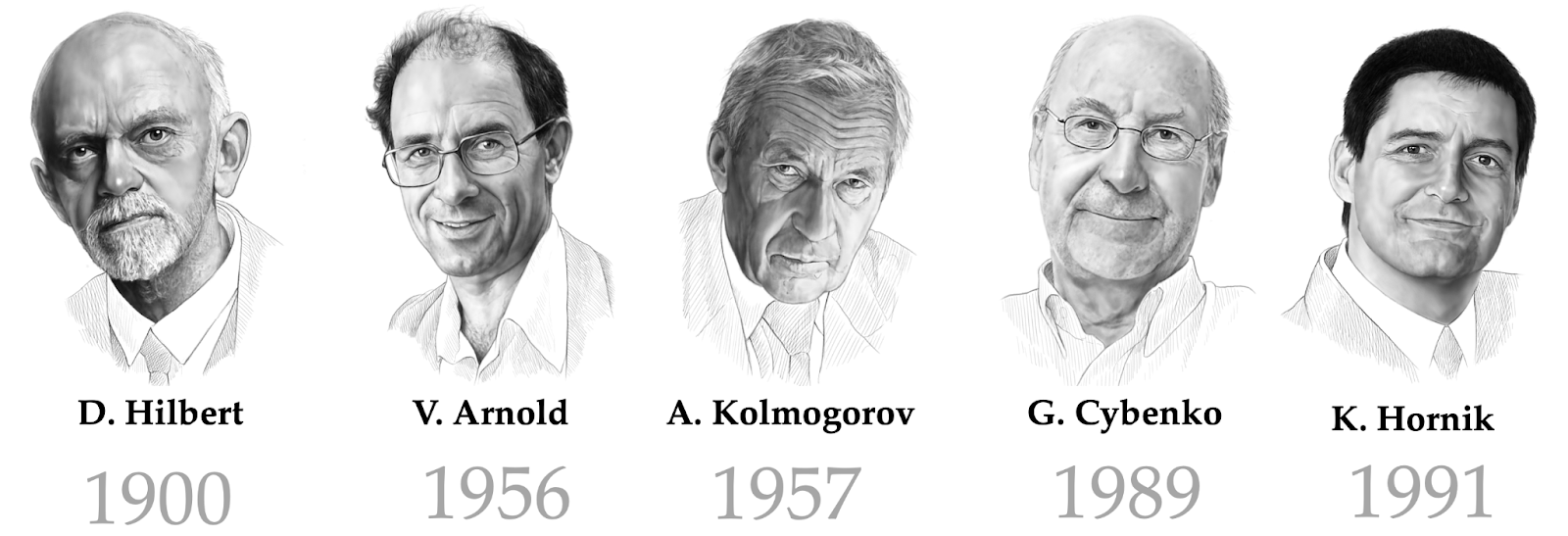
Universal approximation guarantees that we can express functions from a very broad regularity class (continuous functions) by means of a multi-layer neural network. In other words, there exists a neural network with a certain number of neurons and certain weights that approximates a given function mapping from the input to the output space (e.g., from the space of images to the space of labels). However, universal approximation theorems do not tell us how to find such weights. In fact, learning (i.e., finding weights) in neural networks has been a big challenge in the early days.

Rosenblatt showed a learning algorithm only for a single-layer perceptron; to train multi-layer neural networks, Aleksey Ivakhnenko and Valentin Lapa [46] used a layer-wise learning algorithm called ‘group method of data handling.’ This allowed Ivakhnenko [47] to go as deep as eight layers — a remarkable feat for the early 1970s!

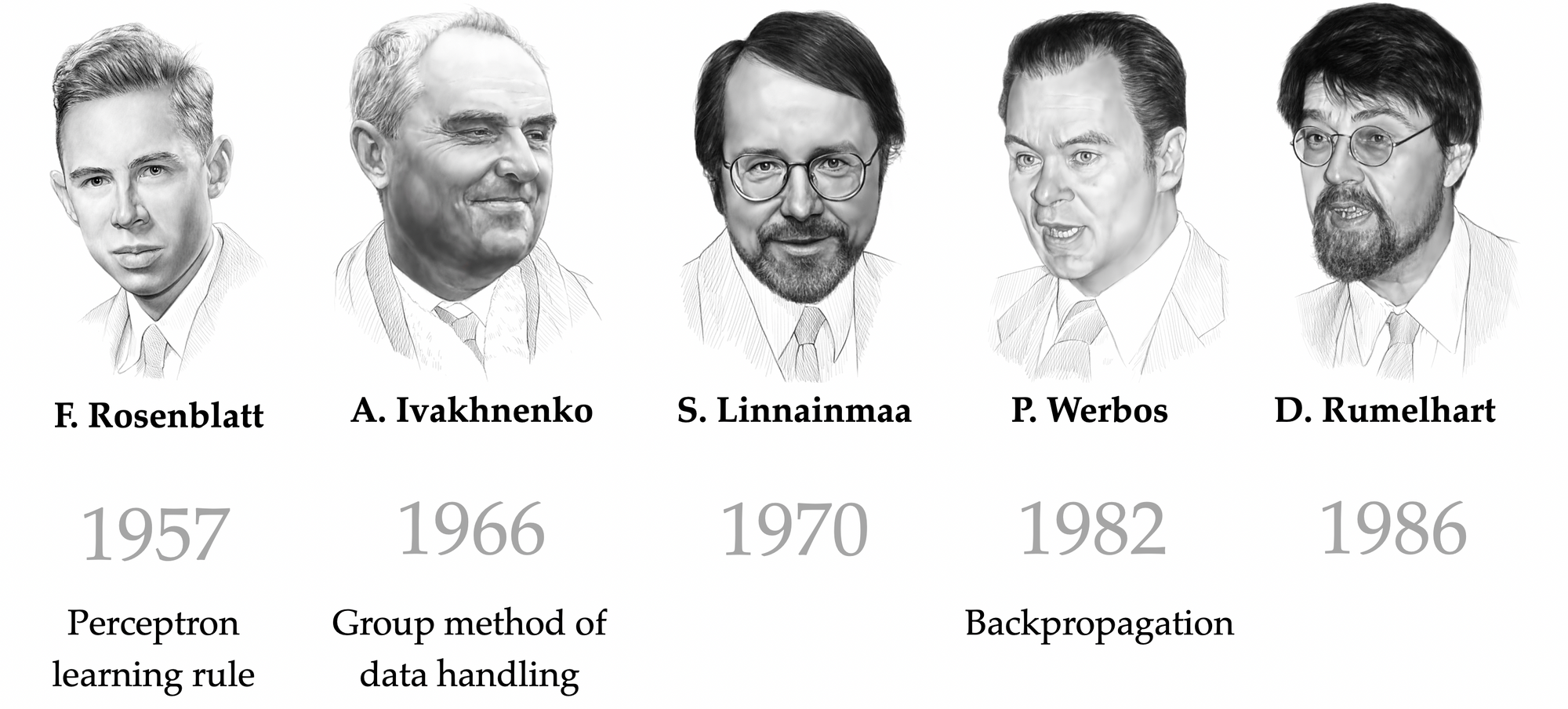
A breakthrough came with the invention of backpropagation, an algorithm using the chain rule to compute the gradient of the weights with respect to the loss function, and allowed to use gradient descent-based optimisation techniques to train neural networks. As of today, this is the standard approach in deep learning. While the origins of backpropagation date back to at least 1960 [48] the first convincing demonstration of this method in neural networks was in the widely cited Nature paper of Rumelhart, Hinton, and Williams [49]. The introduction of this simple and efficient learning method has been a key contributing factor to the return of neural networks to the AI scene in the 1980s and 1990s.

Looking at neural networks through the lens of approximation theory has led some cynics to call deep learning a “glorified curve fitting.” We will let the reader judge how true this maxim is by trying to answer an important question: how many samples (training examples) are needed to accurately approximate a function? Approximation theorists will immediately retort that the class of continuous functions that multilayer perceptrons can represent is obviously way too large: one can pass infinitely many different continuous functions through a finite collection of points [50]. It is necessary to impose additional regularity assumptions such as Lipschitz continuity [51], in which case one can provide a bound on the required number of samples.

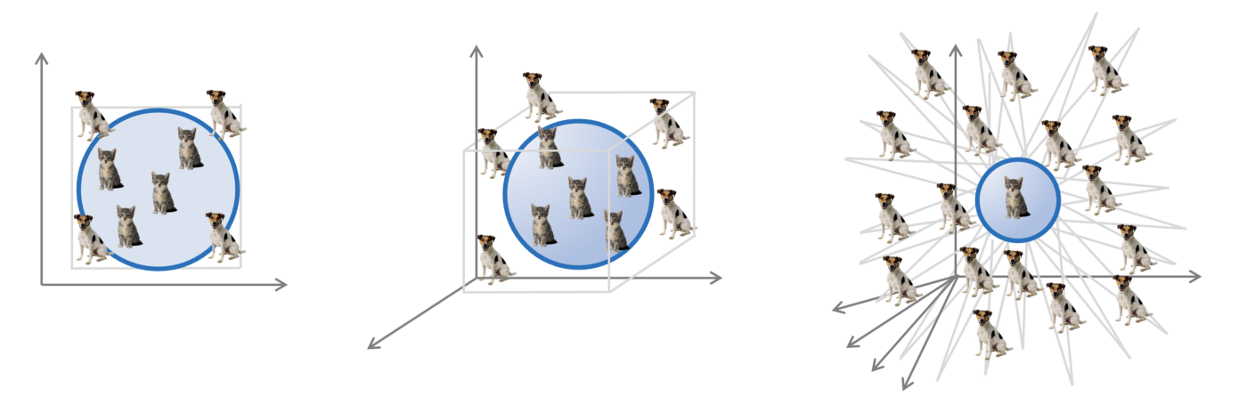
Unfortunately, these bounds scale exponentially with dimension — a phenomenon colloquially known as the ‘curse of dimensionality’ [52] — which is unacceptable in machine learning problems: even small-scale pattern recognition problems, such as image classification, deal with input spaces of thousands of dimensions. If one had to rely only on classical results from approximation theory, machine learning would be impossible. In our illustration, the number of examples of cat and dog images that would be required in theory in order to learn to tell them apart would be way larger than the number of atoms in the universe [53] — there are simply not enough cats and dogs around to do it.

AI Winter is Coming

The struggle of machine learning methods to scale to high dimensions was brought up by the British mathematician Sir James Lighthill in a paper that AI historians call the ‘Lighthill Report’ [54], in which he used the term ‘combinatorial explosion’ and claimed that existing AI methods could only work on toy problems and would become intractable in real-world applications.

“Most workers in AI research and in related fields confess to a pronounced feeling of disappointment in what has been achieved in the past twenty-five years. […] In no part of the field have the discoveries made so far produced the major impact that was then promised.” — Sir James Lighthill (1972)

Since the Lighthill Report was commissioned by the British Science Research Council to evaluate academic research in the field of artificial intelligence, its pessimistic conclusions resulted in funding cuts across the pond. Together with similar decisions by the American funding agencies, this amounted to a wrecking ball for AI research in the 1970s.

Secrets of the Visual Cortex

The next generation of neural networks, which culminated in the triumphant reemergence of deep learning we have witnessed a decade ago, drew their inspiration from neuroscience.

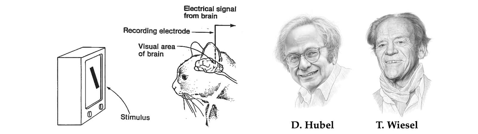
In a series of experiments that would become classical and bring them a Nobel Prize in medicine, the duo of Harvard neurophysiologists David Hubel and Torsten Wiesel [55–56] unveiled the structure and function of a part of the brain responsible for pattern recognition — the visual cortex. By presenting changing light patterns to a cat and measuring the response of its brain cells (neurons), they showed that the neurons in the visual cortex have a multi-layer structure with local spatial connectivity: a cell would produce a response only if cells in its proximity (‘receptive field’ [57]) were activated.

Furthermore, the organisation appeared to be hierarchical, where the responses of ‘simple cells’ reacting to local primitive oriented step-like stimuli were aggregated by ‘complex cells,’ which produced responses to more complex patterns. It was hypothesized that cells in deeper layers of the visual cortex would respond to increasingly complex patterns composed of simpler ones, with a semi-joking suggestion of the existence of a ‘grandmother cell’ [58] that reacts only when shown the face of one’s grandmother.

The Neocognitron

The understanding of the structure of the visual cortex has had a profound impact on early works in computer vision and pattern recognition, with multiple attempts to imitate its main ingredients. Kunihiko Fukushima, at that time a researcher at the Japan Broadcasting Corporation, developed a new neural network architecture [59] “similar to the hierarchy model of the visual nervous system proposed by Hubel and Wiesel,” which was given the name neocognitron [60].

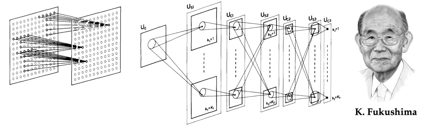
The neocognitron consisted of interleaved S- and C-layers of neurons (a naming convention reflecting its inspiration in the biological visual cortex); the neurons in each layer were arranged in 2D arrays following the structure of the input image (‘retinotopic’), with multiple ‘cell-planes’ (feature maps in modern terminology) per layer. The S-layers were designed to be translationally symmetric: they aggregated inputs from a local receptive field using shared learnable weights, resulting in cells in a single cell-plane having receptive fields of the same function, but at different positions. The rationale was to pick up patterns that could appear anywhere in the input. The C-layers were fixed and performed local pooling (a weighted average), affording insensitivity to the specific location of the pattern: a C-neuron would be activated if any of the neurons in its input are activated.

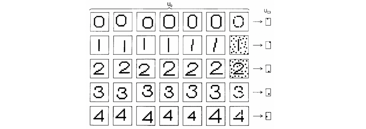
Since the main application of the neocognitron was character recognition, translation invariance [61] was crucial. This property was a fundamental difference from earlier neural networks such as Rosenblatt’s perceptron: in order to use a perceptron reliably, one had to first normalise the position of the input pattern, whereas in the neocognitron, the insensitivity to the pattern position was baked into the architecture. Neocognitron achieved it by interleaving translationally-equivariant local feature extraction layers with pooling, creating a multiscale representation [62]. Computational experiments showed that Fukushima’s architecture was able to successfully recognise complex patterns such as letters or digits, even in the presence of noise and geometric distortions.

Looking from the vantage point of four decades of progress in the field, one finds that the neocognitron already had strikingly many characteristics of modern deep learning architectures: depth (Fukishima simulated a seven-layer network in his paper), local receptive fields, shared weights, and pooling. It even used half-rectifier (ReLU) activation function, which is often believed to be introduced in recent deep learning architectures [63]. The main distinction from modern systems was in the way the network was trained: neocognitron was trained in an unsupervised manner since backpropagation had still not been widely used in the neural network community.

Convolutional Neural Networks

Fukushima’s design was further developed by Yann LeCun, a fresh graduate from the University of Paris [64] with a PhD thesis on the use of backpropagation for training neural networks. In his first post-doctoral position at the AT&T Bell Laboratories, LeCun and colleagues built a system to recognise hand-written digits on envelopes in order to allow the US Postal Service to automatically route mail.

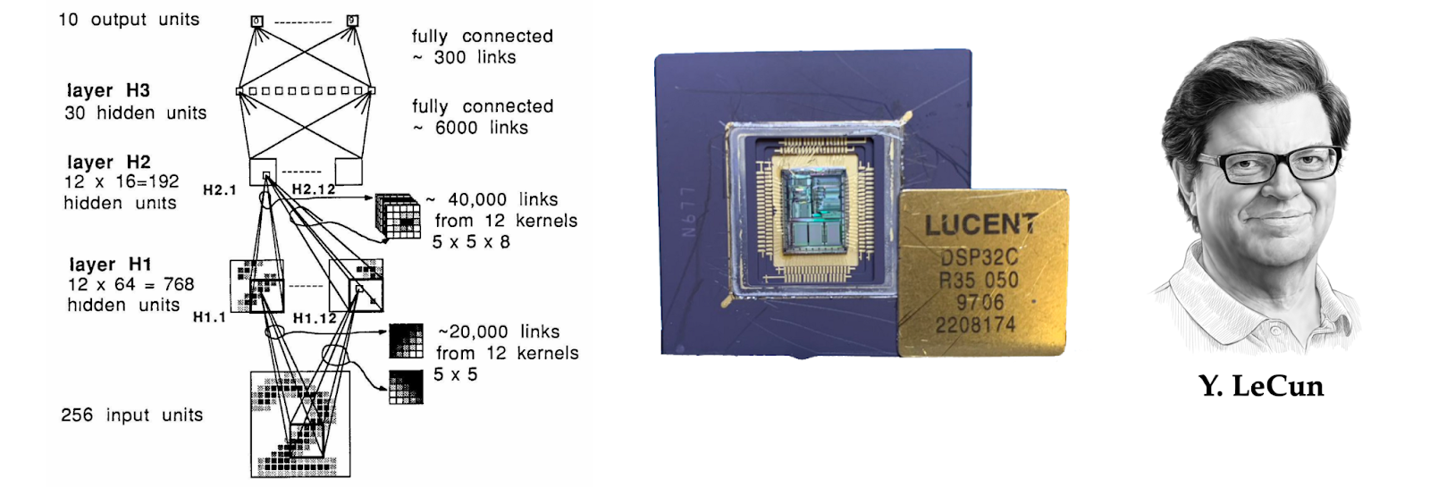
In a paper that is now classical [65], LeCun et al. described the first three-layer convolutional neural network (CNN) [66]. Similarly to the neocognitron, LeCun’s CNN also used local connectivity with shared weights and pooling. However, it forwent Fukushima’s more complex nonlinear filtering (inhibitory connections) in favour of simple linear filters that could be efficiently implemented as convolutions using multiply-and-accumulate operations on a digital signal processor (DSP) [67].

This design choice, departing from the neuroscience inspiration and terminology and moving into the realm of signal processing, would play a crucial role in the ensuing success of deep learning. Another key novelty of CNN was the use of backpropagation for training.

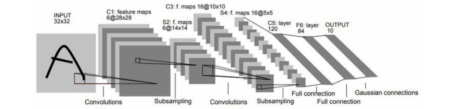
LeCun’s works convincingly showed the power of gradient-based methods for complex pattern recognition tasks and was one of the first practical deep learning-based systems for computer vision. An evolution of this architecture, a CNN with five layers named LeNet-5 as a pun on the author’s name [68], was used by US banks to read handwritten cheques.

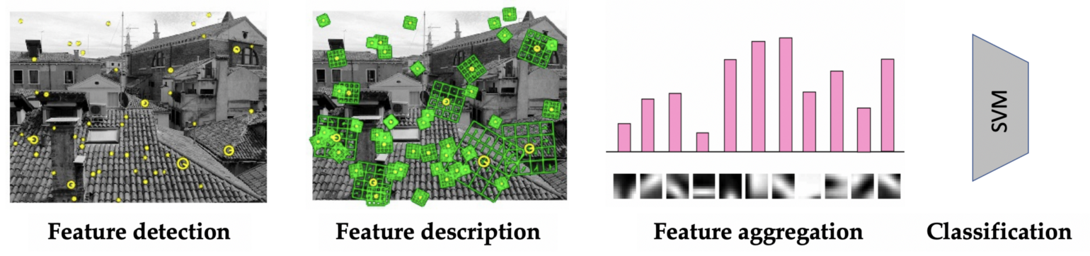
The computer vision research community, however, in its vast majority steered away from neural networks and took a different path. The typical architecture of visual recognition systems of the first decade of the new millennium was a carefully hand-crafted feature extractor (typically detecting interesting points in an image and providing their local description in a way that is robust to perspective transformations and contrast changes [69]) followed by a simple classifier (most often a support vector machine (SVM) and more rarely, a small neural network) [70].

Recurrent Neural Networks, Vanishing gradients, and  LSTMs

While CNNs were mainly applied to modelling data with spatial symmetries such as images, another development was brewing: one that recognises that data is often non-static, but can evolve in a temporal manner as well. The simplest form of temporally-evolving data is a time series consisting of a sequence of steps with a data point provided at each step.

A model handling time-series data hence needs to be capable of meaningfully adapting to sequences of arbitrary length—a feat that CNNs were not trivially capable of. This led to development of Recurrent Neural Networks (RNNs) in the late 1980s and early 1990s [71], the earliest examples of which simply applies a shared update rule distributed through time [72–73]. At every step, the RNN state is updated as a function of the previous state and the current input.

One issue that plagued RNNs from the beginning was the vanishing gradient problem. Vanishing gradients arise in very deep neural networks—of which RNNs are often an instance of, given that their effective depth is equal to the sequence length—with sigmoidal activations is unrolled over many steps, suffers from gradients quickly approaching zero as backpropagation is performed. This effect strongly limits the influence of earlier steps in the sequence to the predictions made in the latter steps.

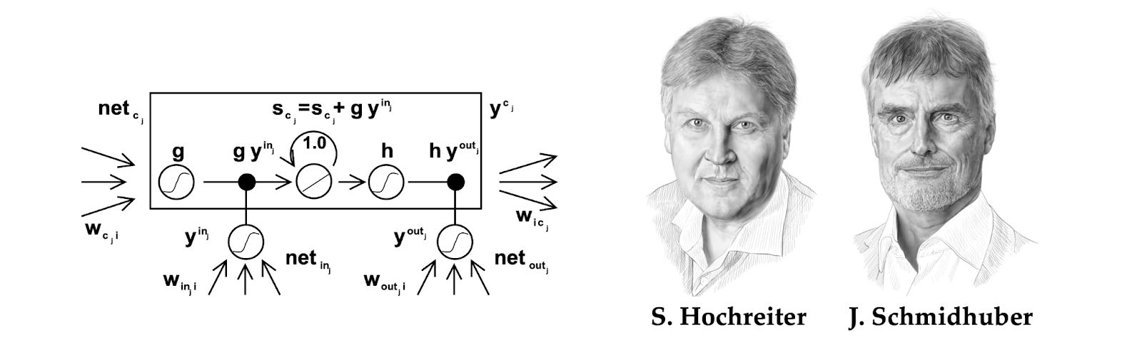
A solution to this problem was first elaborated in Sepp Hochreiter’s Diploma thesis [74](carried out in Munich under the supervision of Jürgen Schmidhuber) in the form of an architecture that was dubbed Long Short-Term Memory (LSTM) [75]. LSTMs combat the vanishing gradient problem by having a memory cell, with explicit gating mechanisms deciding how much of that cell’s state to overwrite at every step—allowing one to learn the degree of forgetting from data (or alternatively, remembering for long time). In contrast, simple RNNs [72–73] perform a full overwrite at every step.

This ability to remember context for long time turned crucial in natural language processing and speech analysis applications, where recurrent models were shown successful applications starting from the early 2000s [76–77]. However, like it happened with CNNs in computer vision, the breakthrough would need to wait for another decade to come.

Gating Mechanisms and Time Warping

In our context, it may not be initially obvious whether recurrent models embody any kind of symmetry or invariance principle similar to the translational invariance we have seen in CNNs. Nearly three decades after the development of RNNs, Corentin Tallec and Yann Ollivier [78] showed that there is a type of symmetry underlying recurrent neural networks: time warping.

Time series have a very important but subtle nuance: it is rarely the case that the individual steps of a time series are evenly spaced. Indeed, in many natural phenomena, we may deliberately choose to take many measurements at some time points and very few (or no) measurements during others. In a way, the notion of “time” presented to the RNN working on such data undergoes a form of warping operation. Can we somehow guarantee that our RNN is “resistant” to time warping, in the sense that we will always be able to find a set of useful parameters for it, regardless of the warping operation applied?

In order to handle time warping with a dynamic rate, the network needs to be able to dynamically estimate how quickly time is being warped (the so-called “warping derivative”) at every step. This estimate is then used to selectively overwrite the RNN’s state. Intuitively, for larger values of the warping derivative, a more strict state overwrite should be performed, as more time has elapsed since.

The idea of dynamically overwriting data in a neural network is implemented through the gating mechanism. Tallec and Ollivier effectively show that, in order to satisfy time warping invariance, an RNN needs to have a gating mechanism. This provides a theoretical justification for gate RNN models, such as the aforementioned LSTMs of Hochreiter and Schmidhuber or the Gated Recurrent Unit (GRU) [79]. Full overwriting used in simple RNNs corresponds to an implicit assumption of a constant time warping derivative equal to 1 – a situation unlikely to happen in most real-world scenarios – which also explains the success of LSTMs.

The Triumph of Deep Learning

As already mentioned, the initial reception of what would later be called “deep learning” had initially been rather lukewarm. The computer vision community, where the first decade of the new century was dominated by handcrafted feature descriptors, appeared to be particularly hostile to the use of neural networks. The balance of power was soon to be changed by the rapid growth in computing power and the amounts of available annotated visual data. It became possible to implement and train increasingly bigger and more complex CNNs that allowed for the addressing of increasingly challenging visual pattern recognition tasks [80], culminating in a Holy Grail of computer vision at that time: the ImageNet Large Scale Visual Recognition Challenge. Established by the American-Chinese researcher Fei-Fei Li in 2009, ImageNet was an annual challenge consisting of the classification of millions of human-labeled images into 1000 different categories.

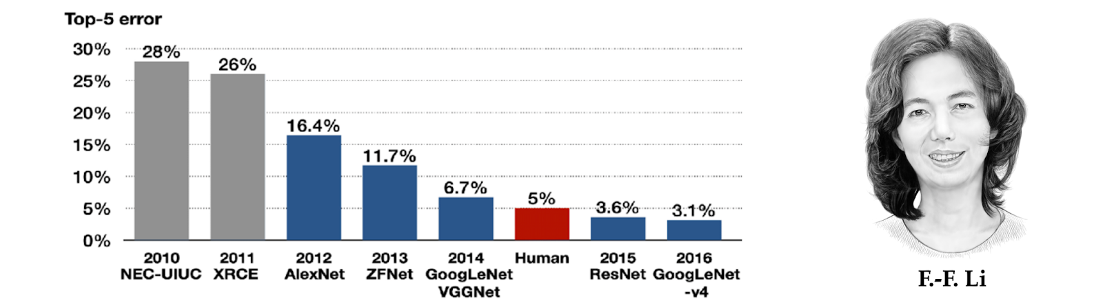
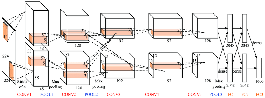
A CNN architecture developed at the University of Toronto by Krizhevsky, Sutskever, and Hinton [81] managed to beat by a large margin [82] all the competing approaches such as smartly engineered feature detectors based on decades of research in the field. AlexNet (as the architecture was called in honour of its developer, Alex Krizhevsky) was significantly bigger in terms of the number of parameters and layers compared to its older sibling LeNet-5 [83], but conceptually the same. The key difference was the use of a graphics processor (GPU) for training [84], now the mainstream hardware platform for deep learning [85].

The success of CNNs on ImageNet became the turning point for deep learning and heralded its broad acceptance in the following decade. A similar transformation happened in natural language processing and speech recognition, which moved entirely to neural network-based approaches during the 2010s; indicatively, Google [86] and Facebook [87] switched their machine translations systems to LSTM-based architectures around 2016-17. Multi-billion dollar industries emerged as a result of this breakthrough, with deep learning successfully used in commercial systems ranging from speech recognition in Apple iPhone to Tesla self-driving cars. More than forty years after the scathing review of Rosenblatt’s work, the connectionists were finally vindicated.

A Needle in a Haystack

If the history of symmetry is tightly intertwined with physics, the history of graph neural networks, a “poster child” of Geometric Deep Learning, has roots in another branch of natural science: chemistry.

Chemistry has historically been — and still is — one of the most data-intensive academic disciplines. The emergence of modern chemistry in the eighteenth century resulted in the rapid growth in the number of known chemical compounds and an early need for their organisation. This role was initially played by periodicals such as the Chemisches Zentralblatt [88] and “chemical dictionaries” like the Gmelins Handbuch der anorganischen Chemie (an early compendium of inorganic compounds first published in 1817 [89]) and Beilsteins Handbuch der organischen Chemie (a similar effort for organic chemistry) — initially published in German, which was one of the dominant language of science in the early 20th century.

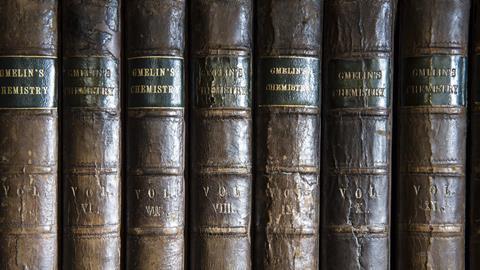
In the English-speaking world, the Chemical Abstracts Service (CAS) was created in 1907 and has gradually become the central repository for the world’s published chemical information [90]. However, the sheer amount of data (the Beilstein alone has grown to over 500 volumes and nearly half a million pages over its lifetime) has quickly made it impractical to print and use such chemical databases.

Since the mid-nineteenth century, chemists have established a universally understood way to refer to chemical compounds through structural formulae, indicating a compound’s atoms, the bonds between them, and even their 3D geometry. But such structures did not lend themselves to easy retrieval.

In the first half of the 20th century, with the rapid growth of newly discovered compounds and their commercial use, the problem of organising, searching, and comparing molecules became of crucial importance: for example, when a pharmaceutical company sought to patent a new drug, the Patent Office had to verify whether a similar compound had been previously deposited.

To address this challenge, several systems for indexing molecules were introduced in the 1940s, forming foundations for a new discipline that would later be called chemoinformatics. One such system, named the ‘GKD chemical cipher’ after the authors Gordon, Kendall, and Davison [91], was developed at the English tire firm Dunlop to be used with early punchcard-based computers [92]. In essence, the GKD cipher was an algorithm for parsing a molecular structure into a string that could be more easily looked up by a human or a computer.

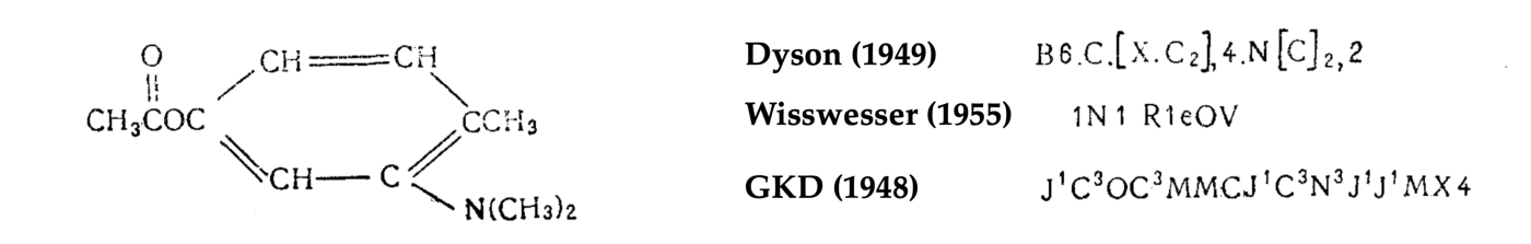
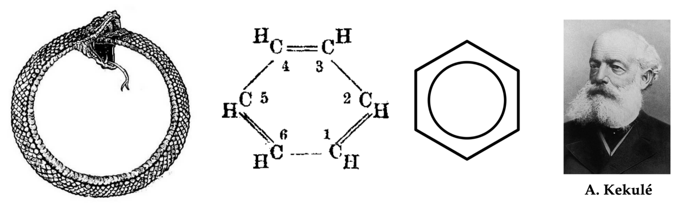
However, the GKD cipher and other related methods [93] were far from satisfactory. In chemical compounds, similar structures often result in similar properties. Chemists are trained to develop intuition to spot such analogies, and look for them when comparing compounds. For example, the association of the benzene ring with odouriferous properties was the reason for the naming of the chemical class of “aromatic compounds” in the 19th century.

On the other hand, when a molecule is represented as a string (such as in the GKD cipher), the constituents of a single chemical structure may be mapped into different positions of the cipher. As a result, two molecules containing a similar substructure (and thus possibly similar properties) might be encoded in very different ways.

This realisation has encouraged the development of “topological ciphers,” trying to capture the structure of the molecule. First works of this kind were done in the Dow Chemicals company [94] and the US Patent Office [95] — both heavy users of chemical databases. One of the most famous such descriptors, known as the ‘Morgan fingerprint’ [96], was developed by Harry Morgan at the Chemical Abstracts Service [97] and used until today.

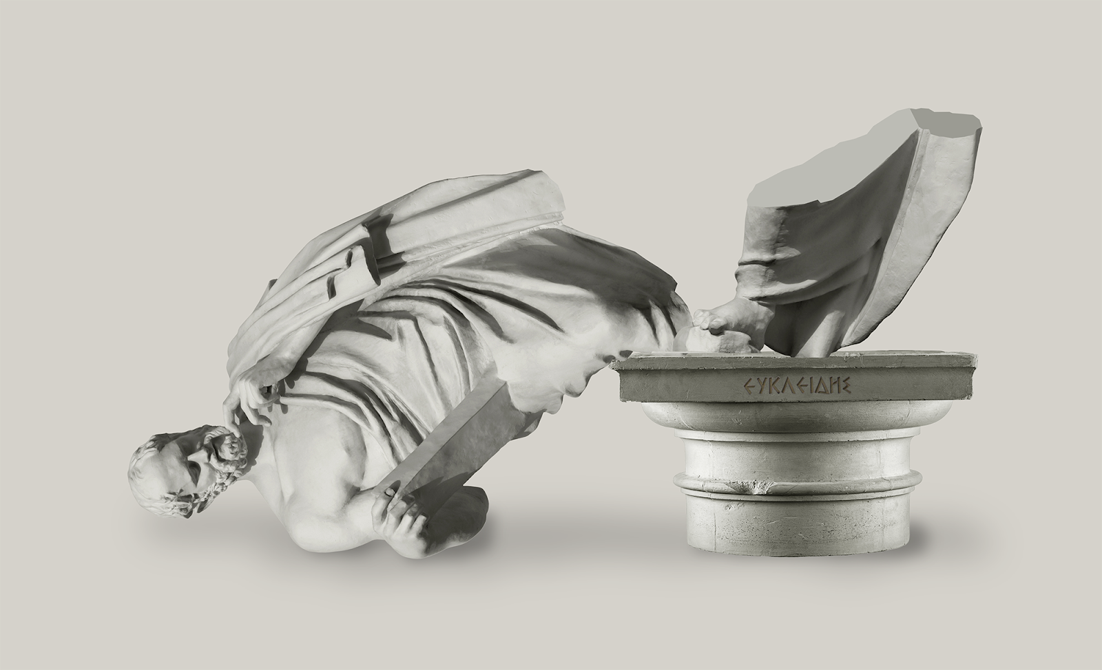
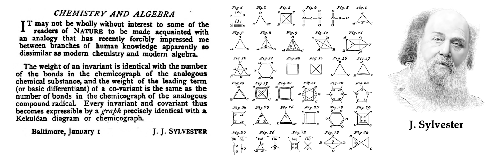
Chemistry Meets Graph Theory

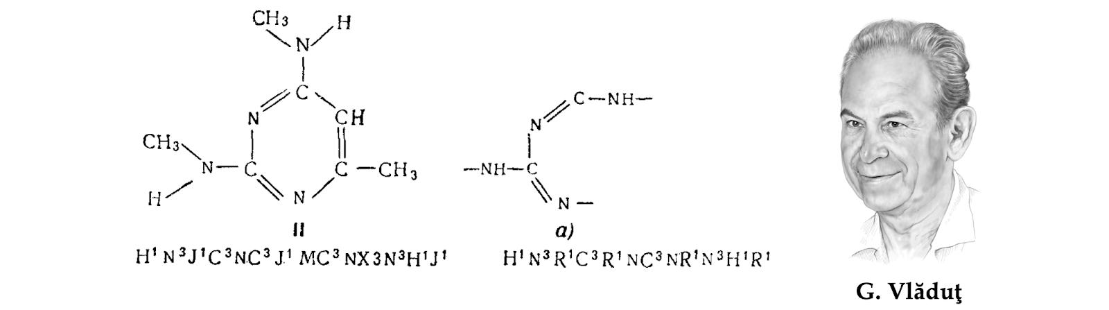
A figure that has played a key role in developing early “structural” approaches for searching chemical databases is the Romanian-born Soviet researcher George Vlăduţ [98]. A chemist by training (he defended a PhD in organic chemistry at the Moscow Mendeleev Institute in 1952), he experienced a traumatic encounter with the gargantuan Beilstein handbook in his freshman years [99]. This steered his research interests towards chemoinformatics [100], a field in which he worked for the rest of his life.

Vlăduţ is credited as one of the pioneers of using graph theory for modeling the structures and reactions of chemical compounds. In a sense, this should not come as a surprise: graph theory has been historically tied to chemistry, and even the term ‘graph’ (referring to a set of nodes and edges, rather than a plot of a function) was introduced by the mathematician James Sylvester in 1878 as a mathematical abstraction of chemical molecules [101].

In particular, Vlăduţ advocated the formulation of molecular structure comparison as the graph isomorphism problem; his most famous work was on classifying chemical reactions as the partial isomorphism (maximum common subgraph) of the reactant and product molecules [102].

Vlăduţ’s work inspired [103] a pair of young researchers, Boris Weisfeiler (an algebraic geometer) and Andrey Lehman [104] (self-described as a “programmer” [105]). In a classical joint paper [106], the duo introduced an iterative algorithm for testing whether a pair of graphs are isomorphic (i.e., the graphs have the same structure up to reordering of nodes), which became known as the Weisfeiler-Lehman (WL) test [107]. Though the two had known each other from school years, their ways parted shortly after their publication and each became accomplished in his respective field [108].

Weisfeiler and Lehman’s initial conjecture that their algorithm solved the graph isomorphism problem (and does it in polynomial time) was incorrect: while Lehman demonstrated it computationally for graphs with at most nine nodes [109], a larger counterexample was found a year later [110] (and in fact, a strongly regular graph failing the WL test called the Shrinkhande graph had been known even earlier [111]).

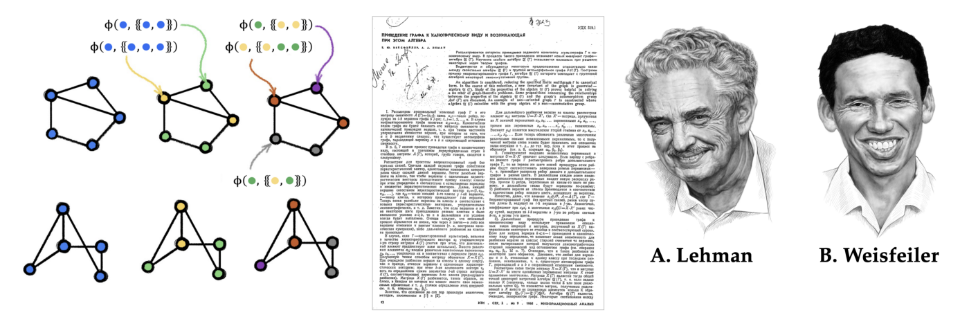
The paper of Weisfeiler and Lehman has become foundational in understanding graph isomorphism. To put their work in historical perspective, one should remember that in the 1960s, complexity theory was still embryonic and algorithmic graph theory was only taking its first baby steps. As Lehman recollected in the late 1990s,

“In the 60s, one could in a matter of days re-discover all the facts, ideas, and techniques in graph isomorphism theory. I doubt that the word ‘theory’ is applicable; everything was at such a basic level.” — Andrey Lehman, 1999

Their result spurred numerous follow-up works, including high-dimensional graph isomorphism tests [112]. In the context of graph neural networks, Weisfeiler and Lehman have recently become household names with the proof of the equivalence of their graph isomorphism test to message passing [113–114].

Early Graph Neural Networks

Though chemists have been using GNN-like algorithms for decades, it is likely that their works on molecular representation remained practically unknown in the machine learning community [115]. We find it hard to pinpoint precisely when the concept of graph neural networks has begun to emerge: partly due to the fact that most of the early work did not place graphs as a first-class citizen, in part because graph neural networks only became practical in the late 2010s, and partly because this field emerged from the confluence of several adjacent research areas.

Early forms of graph neural networks can be traced back at least to the 1990s, with examples including “Labeling RAAM” by Alessandro Sperduti [116], the “backpropagation through structure” by Christoph Goller and Andreas Küchler [117], and adaptive processing of data structures [118–119]. While these works were primarily concerned with operating over “structures” (often trees or directed acyclic graphs), many of the invariances preserved in their architectures are reminiscent of the GNNs more commonly in use today.

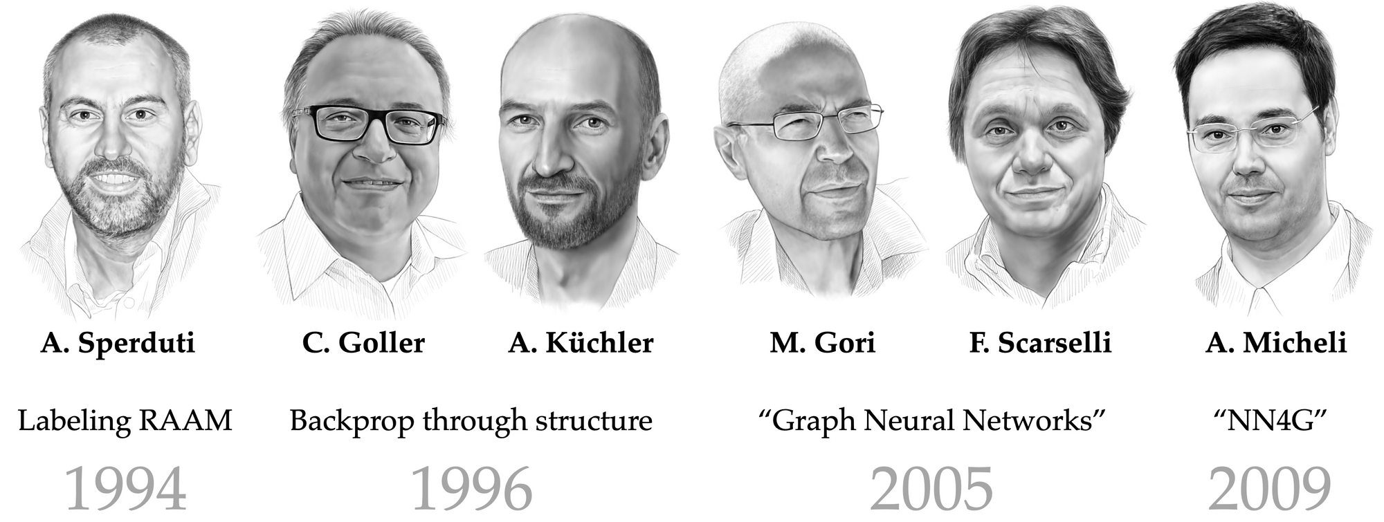
The first proper treatment of the processing of generic graph structures (and the coining of the term ‘graph neural network’) happened after the turn of the 21st century. A University of Siena team led by Marco Gori [120] and Franco Scarselli [121] proposed the first “GNN.” They relied on recurrent mechanisms, required the neural network parameters to specify contraction mappings, and thus computing node representations by searching for a fixed point — this in itself necessitated a special form of backpropagation and did not depend on node features at all. All of the above issues were rectified by the Gated GNN (GGNN) model of Yujia Li [122], which brought many benefits of modern RNNs, such as gating mechanisms [123] and backpropagation through time.

The neural network for graphs (NN4G) proposed by Alessio Micheli around the same time [124] used a feedforward rather than recurrent architecture, in fact resembling more the modern GNNs.

Another important class of graph neural networks, often referred to as “spectral,” has emerged from the work of Joan Bruna and coauthors [125] using the notion of the Graph Fourier transform. The roots of this construction are in the signal processing and computational harmonic analysis communities, where dealing with non-Euclidean signals has become prominent in the late 2000s and early 2010s [126].

Influential papers from the groups of Pierre Vandergheynst [127] and José Moura [128] popularised the notion of “Graph Signal Processing” (GSP) and the generalisation of Fourier transforms based on the eigenvectors of graph adjacency and Laplacian matrices. The graph convolutional neural networks relying on spectral filters by Michaël Defferrard [129] and Thomas Kipf and Max Welling [130] are among the most cited in the field.

It is worth noting that, while the concept of GNNs experienced several independent rederivations in the 2010s arising from several perspectives (e.g., computational chemistry [131,135], digital signal processing [127–128], probabilistic graphical models [132], and natural language processing [133]), the fact that all of these models arrived at different instances of a common blueprint is certainly telling. In fact, it has recently been posited [134] that GNNs may offer a universal framework for processing discretised data. Other neural architectures we have discussed (CNNs or RNNs) may be recovered as special cases of GNNs by inserting appropriate priors into the message passing functions or the graph structure over which the messages are computed.

Back to the Origins

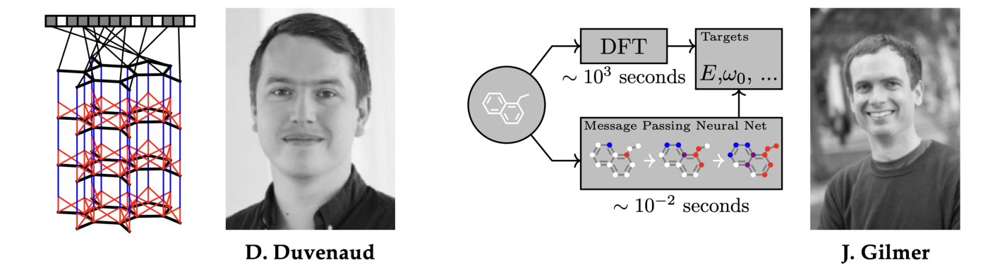
In a somewhat ironic twist of fate, modern GNNs were triumphantly re-introduced to chemistry, a field they originated from, by David Duvenaud [131] as a replacement for handcrafted Morgan’s molecular fingerprints, and by Justin Gilmer [135] in the form of message-passing neural networks equivalent to the Weisfeiler-Lehman test [113–114]. After fifty years, the circle finally closed.

Graph neural networks are now a standard tool in chemistry and have already seen uses in drug discovery and design pipelines. A notable accolade was claimed with the GNN-based discovery of novel antibiotic compounds [136] in 2020. DeepMind’s AlphaFold 2 [137] used equivariant attention (a form of GNN that accounts for the continuous symmetries of the atomic coordinates) in order to address a hallmark problem in structural biology — the problem of protein folding.

In 1999, Andrey Lehman wrote to a mathematician colleague that he had the “pleasure to learn that ‘Weisfeiler-Leman’ was known and still caused interest.” He did not live to see the rise of GNNs based on his work of fifty years earlier. Nor did George Vlăduţ see the realisation of his ideas, many of which remained on paper during his lifetime.

The ‘Erlangen Programme’ of Deep Learning

Our historical overview of the geometric foundations of deep learning has now naturally brought us to the blueprint that underpins this book. Taking Convolutional and Graph Neural Networks as two prototypical examples, at the first glance completely unrelated, we find several common traits. First, both operate on data (images in the case of CNNs or molecules in the case of GNNs) that have underlying geometric domains (respectively, a grid or a graph).

Second, in both cases the tasks have a natural notion of invariance (e.g., to the position of an object in image classification, or the numbering of atoms in a molecule in chemical property prediction) that can be formulated through appropriate symmetry group (translation in the former example and permutation in the latter).

Third, both CNNs and GNNs bake the respective symmetries into their architecture by using layers that interact appropriately with the action of the symmetry group on the input. In CNNs, it comes in the form of convolutional layers whose output transforms in the same way as the input (this property is called translation-equivariance, which is the same as saying that convolution commutes with the shift operator).

In GNNs, it assumes the form of a symmetric message passing function that aggregates neighbouring nodes irrespective of their order. The overall output of a message passing layer transforms regardless of permutations of the input (permutation-equivariant).

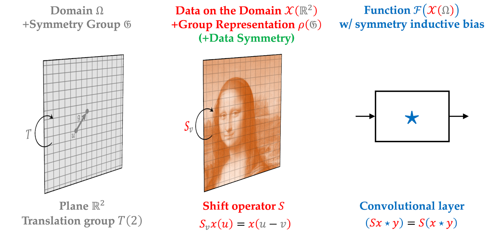
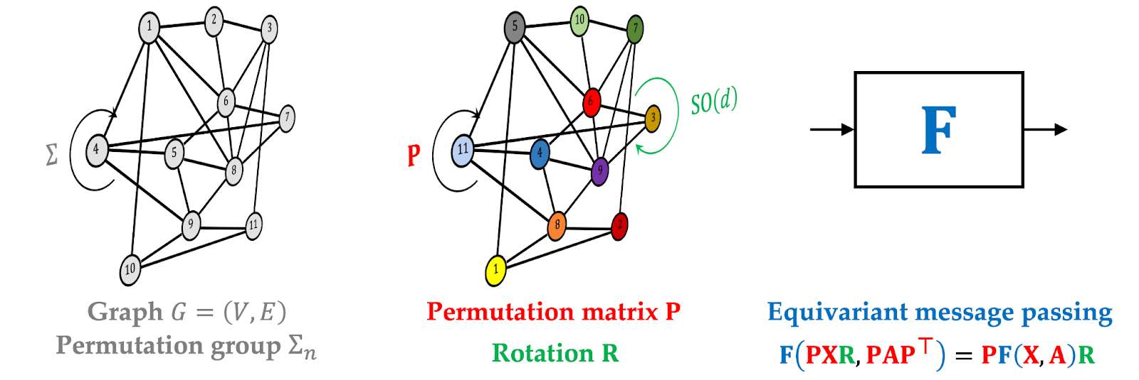
Finally, in some architectural instances, the data are processed in a multi-scale fashion; this corresponds to pooling in CNNs (uniformly sub-sampling the grid that underlies the image) or graph coarsening in some types of GNNs. Overall, this appears to be a very general principle that can be applied to a broad range of problems, types of data, and architectures.

The Geometric Deep Learning Blueprint can be used to derive from first principles some of the most common and popular neural network architectures (CNNs, GNNs, LSTMs, DeepSets, Transformers), which as of today constitute the majority of the deep learning toolkit. All of the above can be obtained by an appropriate choice of the domain and the associated symmetry group.

Further extensions of the Blueprint, such as incorporating additional symmetries of the data in addition to those of the domain, will allow obtaining a new class of equivariant GNN architectures. Such architectures have recently come to the spotlight in the field of biochemistry. In particular, we should mention the groundbreaking success of AlphaFold 2, addressing the long-standing hard  problem of structural biology: predicting protein folding.

Conclusions and Outlook

In conclusion, we will try to provide an outlook as to what might be next in store for Geometric Deep Learning [138]. One obvious question is whether one can automatically discover symmetries or invariances associated with a certain task or dataset, rather than hard-wiring them into the neural network. Several recent works have answered this question positively [139].

Second, the group theoretical framework underlying the Geometric Deep Learning blueprint is a mathematical abstraction, and in reality one may wish to accommodate transformations that do not necessarily form a group. A key concept in this setting is geometric stability [140], which can be interpreted as approximate invariance or equivariance relation [141]. An extension of this notion allows to account for the perturbation of the domain, e.g. changing the connectivity of a graph on which a GNN acts [142].

Third, similarly to how Klein’s blueprint has led to the development of new mathematical disciplines including modern differential geometry, algebraic topology, and category theory, we see exploiting tools and ideas from these fields as one possible next step in the evolution of Geometric Deep Learning. Recent works showed extensions of GNNs using “exotic” constructions from algebraic topology called cellular sheaves [143], offering architectures that are more expressive and whose expressive power can be generalised without resorting to the Weisfeiler-Lehman formalism [145]. Another line of works uses constructions from Category Theory to extend our blueprint beyond groups [146].

Finally, taking note of the deep connections between geometry and physics, we believe that interesting insights can be brought into the analysis and design of Geometric Deep Learning architectures (in particular, GNNs) by realising them as discretised physical dynamical systems [146–148].

–

Michael Bronstein is the DeepMind Professor of AI at the University of Oxford. Joan Bruna Joan Bruna is an Associate Professor of Data Science, Computer Science and Mathematics (affiliated) in the Courant Institute of Mathematical Sciences and the Center for Data Science, New York University. He is also a visiting scholar at the Flatiron Institute, part of the Simons Foundation. . Taco Cohen is Machine Learning Researcher and Principal Engineer at Qualcomm AI Research. Petar Veličković is Staff Research Scientist at DeepMind and Affiliated Lecturer at the University of Cambridge. The four authors are currently working on a book “Geometric Deep Learning” that will appear with MIT Press.

We are grateful to Ihor Gorskiy for the hand-drawn portraits and to Tariq Daouda for editing this post.

—

[1] H. Weyl, Symmetry (1952), Princeton University Press.

[2] Fully titled Strena, Seu De Nive Sexangula (’New Year’s gift, or on the Six-Cornered Snowflake’) was, as suggested by the title, a small booklet sent by Kepler in 1611 as a Christmas gift to his patron and friend Johannes Matthäus Wackher von Wackenfels.

[3] P. Ball, In retrospect: On the six-cornered snowflake (2011), Nature 480 (7378):455–455.

[4] Galois famously described the ideas of group theory (which he considered in the context of finding solutions to polynomial equations) and coined the term “group” (groupe in French) in a letter to a friend written on the eve of his fatal duel. He asked to communicate his ideas to prominent mathematicians of the time, expressing the hope that they would be able to “‘decipher all this mess’” (“‘déchiffrer tout ce gâchis”). Galois died two days later from wounds suffered in the duel aged only 20, but his work has been transformational in mathematics.

[5] See biographic notes in R. Tobies, Felix Klein — Mathematician, Academic Organizer, Educational Reformer (2019), The Legacy of Felix Klein 5–21, Springer.

[6] Omar Khayyam is nowadays mainly remembered as a poet and author of the immortal line “‘a flask of wine, a book of verse, and thou beside me.”

[7] The publication of Euclides vindicatus required the approval of the Inquisition, which came in 1733 just a few months before the author’s death. Rediscovered by the Italian differential geometer Eugenio Beltrami in the nineteenth century, Saccheri’s work is now considered an early almost-successful attempt to construct hyperbolic geometry.

[8] Poncelet was a military engineer and participant in Napoleon’s Russian campaign, where he was captured and held as a prisoner until the end of the war. It was during this captivity period that he wrote the Traité des propriétés

projectives des figures (‘Treatise on the projective properties of figures,’ 1822) that revived the interest in projective geometry. Earlier foundation work on this subject was done by his compatriot Gérard Desargues in 1643.

[9] In the 1832 letter to Farkas Bolyai following the publication of his son’s results, Gauss famously wrote: “To praise it would amount to praising myself. For the entire content of the work coincides almost exactly with my own meditations which have occupied my mind for the past thirty or thirty-five years.” Gauss was also the first to use the term ‘non-Euclidean geometry,’ referring strictu sensu to his own construction of hyperbolic geometry. See

R. L. Faber, Foundations of Euclidean and non-Euclidean geometry (1983), Dekker and the blog post in Cantor’s Paradise.

[10] Н. И. Лобачевский, О началах геометрии (1829).

[11] A model for hyperbolic geometry known as the pseudosphere, a surface with constant negative curvature, was shown by Eugenio Beltrami, who also proved that hyperbolic geometry was logically consistent. The term ‘hyperbolic geometry’ was introduced by Felix Klein.

[12] For example, an 1834 pamphlet signed only with the initials “S.S.” (believed by some to belong to Lobachevsky’s long-time opponent Ostrogradsky) claimed that Lobachevsky made “an obscure and heavy theory” out of “the lightest and clearest chapter of mathematics, geometry,” wondered why one would print such “ridiculous fantasies,” and suggested that the book was a “joke or satire.”

[13] A. F. Möbius, Der barycentrische Calcul (1827).

[14] B. Riemann, Über die Hypothesen, welche der Geometrie zu Grunde liegen (1854). See English translation.

[15] According to a popular belief, repeated in many sources including Wikipedia, the Erlangen Programme was delivered in Klein’s inaugural address in October 1872. Klein indeed gave such a talk (though on December 7, 1872), but it was for a non-mathematical audience and concerned primarily his ideas of mathematical education; see[4]. The name “Programme” comes from the subtitle of the published brochure [17], Programm zum Eintritt in die philosophische Fakultät und den Senat der k. Friedrich-Alexanders-Universität zu Erlangen (‘Programme for entry into the Philosophical Faculty and the Senate of the Emperor Friedrich-Alexander University of Erlangen’).

[16] S. Eilenberg and S. MacLane, General theory of natural equivalences (1945), Trans. AMS 58(2):231–294. See also J.-P. Marquis, Category Theory and Klein’s Erlangen Program (2009), From a Geometrical Point of View 9–40, Springer. Concepts from category theory can also be used to explain deep learning architectures even beyond the lens of symmetry, see e.g. P. De Haan et al., Natural graph networks (2020), NeurIPS.

[17] F. Klein, Vergleichende Betrachtungen über neuere geometrische Forschungen (1872). See English translation.

[18] At the time, Göttingen was Germany’s and the world’s leading centre of mathematics. Though Erlangen is proud of its association with Klein, he stayed there for only three years, moving in 1875 to the Technical University of Munich (then called Technische Hochschule), followed by Leipzig (1880), and finally settling down in Göttingen from 1886 until his retirement.

[19] Emmy Noether is rightfully regarded as one of the most important women in mathematics and one of the greatest mathematicians of the twentieth century. She was unlucky to be born and live in an epoch when the academic world was still entrenched in the medieval beliefs of the unsuitability of women for science. Her career as one of the few women in mathematics having to overcome prejudice and contempt was a truly trailblazing one. It should be said to the credit of her male colleagues that some of them tried to break the rules. When Klein and David Hilbert first unsuccessfully attempted to secure a teaching position for Noether at Göttingen, they met fierce opposition from the academic hierarchs. Hilbert reportedly retorted sarcastically to concerns brought up in one such discussion: “I do not see that the sex of the candidate is an argument against her admission as a Privatdozent. After all, the Senate is not a bathhouse”(see C. Reid, Courant in Göttingen and New York: The Story of an Improbable Mathematician (1976), Springer). Nevertheless, Noether enjoyed great esteem among her close collaborators and students, and her male peers in Göttingen affectionately referred to her as “Der Noether,” in the masculine (see C. Quigg, Colloquium: A Century of Noether’s Theorem (2019), arXiv:1902.01989).

[20] E. Noether, Invariante Variationsprobleme (1918), König Gesellsch. d. Wiss. zu Göttingen, Math-Phys. 235–257. See English translation.

[21] J. C. Maxwell, A dynamical theory of the electromagnetic field (1865), Philosophical Transactions of the Royal Society of London 155:459–512.

[22] Weyl first conjectured (incorrectly) in 1919 that invariance under the change of scale or “gauge” was a local symmetry of electromagnetism. The term gauge, or Eich in German, was chosen by analogy to the various track gauges of railroads. After the development of quantum mechanics, he modified the gauge choice by replacing the scale factor with a change of wave phase in iH. Weyl, Elektron und gravitation (1929), Zeitschrift für Physik 56 (5–6): 330–352. See N. Straumann, Early history of gauge theories and weak interactions (1996), arXiv:hep-ph/9609230.

[23] C.-N. Yang and R. L. Mills, Conservation of isotopic spin and isotopic gauge invariance (1954), Physical Review 96 (1):191.

[24] The term “Standard Model” was coined by A. Pais and S. B. Treiman, How many charm quantum numbers are there? (1975), Physical Review Letters 35(23):1556–1559. The Nobel laureate Frank Wilczek is known for the criticism of this term, since, in his words “‘model’ connotes a disposable makeshift, awaiting replacement by the ‘real thing’” whereas “‘standard’ connotes ‘conventional’ and hints at superior wisdom.” Instead, he suggested renaming the Standard Model into “Core Theory.”

[25] P. W. Anderson, More is different (1972), Science 177 (4047): 393–396.

[26] Our review is by no means a comprehensive one and aims at highlighting the development of geometric aspects of deep learning. Our choice to focus on CNNs, RNNs and GNNs is merely pedagogical and does not imply there have not been other equally important contributions in the field.

[27] W. S. McCulloch and W. Pitts, A logical calculus of the ideas immanent in nervous activity (1943), The Bulletin of Mathematical Biophysics 5(4):115–133.

[28] The Dartmouth Summer Research Project on Artificial Intelligence was a 1956 summer workshop at Dartmouth College that is considered to be the founding event of the field of artificial intelligence.

[29] F. Rosenblatt, The perceptron, a perceiving and recognizing automaton (1957), Cornell Aeronautical Laboratory. The name is a portmanteau of ‘perception’ and the Greek suffix -τρον denoting an instrument.

[30] M. Minsky and S. A. Papert, Perceptrons: An introduction to computational geometry (1969), MIT Press.

[31] That is why we can only smile at similar recent claims about the ‘consciousness’ of deep neural networks: אין כל חדש תחת השמש.

[32] Sic in quotes, as “pattern recognition” has not yet become an official term.

[33] Specifically, Minsky and Papert considered binary classification problems on a 2D grid (‘retina’ in their terminology) and a set of linear threshold functions. While the inability to compute the XOR function is always brought up as the main point of criticism in the book, much of the attention was dedicated to geometric predicates such as parity and connectedness. This problem is alluded to on the cover of the book, which is adorned by two patterns: one is connected, and another one is not. Even for a human, it is very difficult to determine which is which.

[34] E. Kussul, T. Baidyk, L. Kasatkina, and V. Lukovich, Rosenblatt perceptrons for handwritten digit recognition (2001), IJCNN showed that Rosenblatt’s 3-layer perceptrons implemented on the 21st-century hardware achieve an accuracy of 99.2% on the MNIST digit recognition task, which is on par with modern models.

[35] Hilbert’s Thirteenth Problem is one of the 23 problems compiled by David Hilbert in 1900 and entailing the proof of whether a solution exists for all 7th-degree equations using continuous functions of two arguments. Kolmogorov and his student Arnold showed a solution of a generalised version of this problem, which is now known as the Arnold–Kolmogorov Superposition Theorem.

[36] В. И. Арнольд, О представлении непрерывных функций нескольких переменных суперпозициями непрерывных функций меньшего числа переменных (1956), Доклады Академии Наук СССР 108:179–182.

[37] В. И. Арнольд, О функции трех переменных (1957), Доклады Академии Наук СССР 114:679–681.

[38] H. D. Block, A review of “Perceptrons: An introduction to computational geometry” (1970), Information and Control 17(5): 501–522.

[39] Computational Geometry has subject code I.3.5 in the ACM Computing Classification System.

[40] S.-I. Amari, Feature spaces which admit and detect invariant signal transformations (1978), Joint Conference on Pattern Recognition.

[41] T. Sejnowski et al., Learning symmetry groups with hidden units: Beyond the perceptron (1986), Physica D: Nonlinear Phenomena 22(1–3):260–275.

[42] J. Shawe-Taylor, Building symmetries into feedforward networks (1989), ICANN.

[43] J. Shawe-Taylor, Symmetries and discriminability in feedforward network architectures (1993), IEEE Trans. Neural Networks 4(5): 816–826.

[44] G. Cybenko, Approximation by superpositions of a sigmoidal function (1989), Mathematics of Control, Signals and Systems 2(4):303–314.

[45] K. Hornik, Approximation capabilities of multilayer feedforward networks (1991) Neural Networks 4(2):251–257.

[46] А. Г. Ивахненко, В. Г. Лапа, Кибернетические предсказывающие устройства (1965), Наукова думка.

[47] A. Ivakhnenko, Polynomial theory of complex systems (1971), IEEE Trans. Systems, Man, and Cybernetics 4:364–378.

[48] Backpropagation is based on the chain rule of differentiation that itself goes back to the co-inventor of differential calculus Gottfried Wilhelm von Leibniz in 1676. A precursor of backpropagation was used by H. J. Kelley, Gradient theory of optimal flight paths (1960), Ars Journal 30(10):947–954 to perform optimisation of complex nonlinear multi-stage systems. Efficient backpropagation that is still in use today was described in the Finnish master’s thesis of S. Linnainmaa, Algoritmin kumulatiivinen pyoristysvirhe yksittaisten pyoristysvirheiden taylor-kehitelmana (1970), University of Helsinki. The earliest use in neural networks is due to P. J. Werbos, Applications of advances in nonlinear sensitivity analysis (1982), System Modeling and Optimization 762–770, Springer, which is usually cited as the origin of the method. See J. Schmidhuber, Deep learning in neural networks: An overview (2015), Neural Networks 61:85–117.

[49] D. E. Rumelhart, G. E. Hinton, and R. J. Williams, Learning representations by back-propagating errors (1986), Nature 323(6088):533–536.

[50] There are even examples of continuous nowhere differentiable functions such as the construction of Weierstrass (1872).

[51] Roughly, Lipschitz-continuous functions do not arbitrarily shrink or expand the distance between points on the domain. For differentiable functions, Lipschitz continuity can be expressed as an upper bound on the norm of the gradient, implying that the function does not ‘jump’ too abruptly.

[52] The first to use the term was Richard Bellman in the preface of his 1957 book Dynamic Programming, where he refers to dimensionality as “a curse which has hung over the head of the physicist and astronomer for many a year.”

[53] The number of protons in the observable universe, known as the Eddington number, is estimated at 10⁸⁰.

[54] J. Lighthill, Artificial intelligence: A general survey (1973) Artificial Intelligence 1–21, Science Research Council London.

[55] D. H. Hubel and T. N. Wiesel, Receptive fields of single neurones in the cat’s striate cortex (1959), The Journal of Physiology 148(3):574.

[56] D. H. Hubel and T. N. Wiesel, Receptive fields, binocular interaction and functional architecture in the cat’s visual cortex (1962), The Journal of Physiology 160(1):106.

[57] The term ‘receptive field’ predates Hubel and Wiesel and was used by neurophysiologists from the early twentieth century, see C. Sherrington, The integrative action of the nervous system (1906), Yale University Press.

[58] The term ‘grandmother cell’ is likely to have first appeared in Jerry Lettvin’s course ‘Biological Foundations for Perception and Knowledge’ held at MIT in 1969. A similar concept of ‘gnostic neurons’ was introduced two years earlier in a book by Polish neuroscientist J. Konorski, Integrative activity of the brain; an interdisciplinary approach (1967). See C. G. Gross, Genealogy of the “grandmother cell” (2002), The Neuroscientist 8(5):512–518.

[59] K. Fukushima, Neocognitron: A self-organizing neural network model for a mechanism of pattern recognition unaffected by shift in position (1980), Biological Cybernetics 36:196– 202. The shift-invariance property is alluded to in the title.

[60] Often misspelled as ‘neurocognitron’, the name ‘neocognitron’ suggests it was an improved version of an earlier architecture of K. Fukushima, Cognitron: a self-organizing multilayered neural network (1975), Biological Cybernetics 20:121–136.

[61] In the words of the author himself, having an output that is “dependent only upon the shape of the stimulus pattern, and is not affected by the position where the pattern is presented.”

[62] We refer to this principle as scale separation, which, like symmetry, is a fundamental property of many physical systems. In convolutional architectures, scale separation allows dealing with a broader class of geometric transformations in addition to translations.

[63] ReLU-type activations date back to at least the 1960s and have been previously employed in K. Fukushima, Visual feature extraction by a multilayered network of analog threshold elements (1969), IEEE Trans. Systems Science and Cybernetics 5(4):322–333.

[64] Université Pierre-et-Marie-Curie, today part of the Sorbonne University.

[65] Y. LeCun et al., Backpropagation applied to handwritten zip code recognition (1989) Neural Computation 1(4):541–551.

[66] In LeCun’s 1989 paper, the architecture was not named; the term ‘convolutional neural network’ or ‘convnet’ would appear in a later paper in 1998 [68].

[67] LeCun’s first CNN was trained on a CPU (a SUN-4/250 machine). However, the image recognition system using a trained CNN was run on AT&T DSP-32C (a second-generation digital signal processor with 256KB of memory capable of performing 125m floating-point multiply-and-accumulate operations per second with 32-bit precision), achieving over 30 classifications per second.

[68] Y. LeCun et al., Gradient-based learning applied to document recognition (1998), Proc. IEEE 86(11): 2278–2324.

[69] One of the most popular feature descriptors was the scale-invariant feature transform (SIFT), introduced by David Lowe in 1999. The paper was rejected multiple times and appeared only five years later, D. G. Lowe, Distinctive image features from scale-invariant keypoints, (2004) IJCV 60(2):91–110. It is one of the most cited computer vision papers.

[70] A prototypical approach was “bag-of-words” representing images as histograms of vector-quantised local descriptors. See e.g. J. Sivic and A. Zisserman, Video Google: A text retrieval approach to object matching in videos (2003), ICCV.

[71] As it often happens, it is hard to point to the first RNN design. Recurrence in neural networks was already described McCulloch and Pitts [27], who noted that “the nervous system contains many circular paths” and referred to “precise specification of these implications by means of recursive functions and determination of those that can be embodied in the activity of nervous nets.” The book M. Minsky, Computation: Finite and Infinite Machines (1967), Prentice-Hall, uses McCulloch-Pitts neurons and calls recurrent architectures “networks with cycles.” D. E. Rumelhart, G. E. Hinton, and R. J. Williams, Learning internal representations by error propagation (1985), ICS Report (an earlier version of the famous Nature paper [49] by the same authors) contains generalisations for learning in RNNs, which are named “recurrent nets,” and credits to Minsky and Papert [30].

[72] M. I. Jordan, Serial Order: A parallel distributed processing approach (1986), ICS Report.

[73] J. L. Elman, Finding structure in time (1990), Cognitive Science 14(2):179–211.

[74] S. Hochreiter. Untersuchungen zu dynamischen neuronalen Netzen. Diploma thesis, TUM, 1991. The paper presenting LSTMs was initially rejected from NIPS in 1995 and appeared only two years later as S. Hochreiter, J. Schmidhuber, Long Short-Term Memory (1997) Neural Computation 9(8):1735-1780.

[75] See also Y. Bengio et al., Learning long-term dependencies with gradients is difficult (1994), Trans. Neural Networks 5(2):157–166 and  R. Pascanu et al., On the difficulty of training recurrent neural networks (2003), ICML.

[76] F. A. Gers and J. Schmidhuber. LSTM recurrent networks learn simple context free and context sensitive languages (2001), IEEE Transactions on Neural Networks 12(6):1333-1340.

[77] A. Graves et al., Biologically plausible speech recognition with LSTM neural nets (2004), Workshop on Biologically Inspired Approaches to Advanced Information Technology.

[78] C. Tallec and Y. Ollivier, Can recurrent neural networks warp time? (2018), ICLR.

[79] K. Cho et al., On the properties of neural machine translation: Encoder–decoder approaches (2014), ACL.

[80] In particular, the group of Jürgen Schmidhuber developed deep large-scale CNN models that won several vision competitions, including Chinese character recognition (D. C. Ciresan et al., Deep big simple neural nets for handwritten digit recognition (2010), Neural Computation 22(12):3207–3220) and traffic sign recognition (D. C. Ciresan et al., Multi-column deep neural network for traffic sign classification, Neural Networks 32:333–338, 2012).

[81] A. Krizhevsky, I. Sutskever, and G. E. Hinton, ImageNet classification with deep convolutional neural networks (2012), NIPS.

[82] AlexNet achieved an error over 10.8% smaller than the runner up.

[83] AlexNet had eleven layers was trained on 1.2M images from ImageNet (for comparison, LeNet-5 had five layers and was trained on 60K MNIST digits). Additional important changes compared to LeNet-5 were the use of ReLU activation (instead of tanh), maximum pooling, dropout regularisation, and data augmentation.

[84] It took nearly a week to train AlexNet on a pair of Nvidia GTX 580 GPUs, capable of ~200G FLOP/sec.

[85] Though GPUs were initially designed for graphics applications, they turned out to be a convenient hardware platform for general-purpose computations (“GPGPU”). First such works showed linear algebra algorithms, see e.g. J. Krüger and R. Westermann, Linear algebra operators for GPU implementation of numerical algorithms (2003), ACM Trans. Graphics 22(3):908–916. The first use of GPUs for neural networks was by K.-S. Oh and K. Jung, GPU implementation of neural networks (2004), Pattern Recognition 37(6):1311–1314, predating AlexNet by nearly a decade.

[86] C. Metz, An infusion of AI makes Google Translate more powerful than ever (2016), Wired.

[87] A. Sidorov, ​​Transitioning entirely to neural machine translation (2017), Meta Engineering Blog.

[88] Originally Pharmaceutisches Central-Blatt, it was the oldest German chemical abstracts journal published between 1830 and 1969.

[89] Named after Leopold Gmelin who published the first version in 1817, the Gmelins Handbuch last print edition appeared in the 1990s. The database currently contains 1.5 million compounds and 1.3 million different reactions discovered between 1772 and 1995.

[90] In 1906, the American Chemical Society authorised the publication of Chemical Abstracts, charging it with the mission of abstracting the world’s literature of chemistry and assigning an initial budget of fifteen thousand dollars. The first publication appeared in 1907 under the stewardship of William Noyes. Over a century since its establishment, the CAS contains nearly 200 million organic and inorganic substances disclosed in publications since the early 1800s.

[91] M. Gordon, C. E. Kendall, and W. H. T. Davison, Chemical Ciphering: a Universal Code as an Aid to Chemical Systematics (1948), The Royal Institute of Chemistry.

[92] A special purpose computer (“Electronic Structural Correlator”), to be used in conjunction with a punch card sorter, was proposed by the Gordon-Kendall-Davison group in connection with their system of chemical ciphering, but never built.

[93] There were several contemporaneous systems that competed with each other, see W. J. Wisswesser, 107 Years of line-formula notations (1968), J. Chemical Documentation 8(3):146–150.

[94] A. Opler and T. R. Norton, A Manual for programming computers for use with a mechanized system for searching organic compounds (1956), Dow Chemical Company.

[95] L. C. Ray and R. A. Kirsch, Finding chemical records by digital computers (1957), Science 126(3278):814–819.

[96] H. L. Morgan. The generation of a unique machine description for chemical structures — a technique developed at Chemical Abstracts Service (1965), J. Chemical Documentation 5(2):107–113.

[97] Not much biographical information is available about Harry Morgan. According to an obituary, after publishing his famous molecular fingerprints paper, he moved to a managerial position at IBM, where he stayed until retirement in 1993. He died in 2007.

[98] In Russian publications, Vlăduţ’s name appeared as Георгий Эмильевич Влэдуц, transliterated as Vleduts or Vladutz. We stick here to the original Romanian spelling.

[99] According to Vladimir Uspensky, Vlăduţ told the anecdote of his encounter with Beilstein in the first lecture of his undergraduate course on organic chemistry during his Patterson-Crane Award acceptance speech at the American Chemical Society. See В. А. Успенский, Труды по нематематике (2002).

[100] Г. Э. Влэдуц, В. В. Налимов, Н. И. Стяжкин, Научная и техническая информация как одна из задач кибернетики (1959), Успехи физических наук 69:1.

[101] J. J. Sylvester, Chemistry and algebra (1878), Nature 17:284.

[102] G. E. Vleduts, Concerning one system of classification and codification of organic reactions (1963), Information Storage and Retrieval 1:117–146.

[103] We were unable to find solid proof of whether or how Weisfeiler and Lehman interacted with Vlăduţ, as most of the people who had known both are now dead. The strongest evidence is a comment in their classical paper [106] acknowledging Vlăduţ for “formulating the problem” (“авторы выражают благодарность В. Э. Влэдуцу за постановку задачи”). It is also certain that Weisfeiler and Lehman were aware of the methods developed in the chemical community, in particular the method of Morgan [96], whom they cited in their paper as a “similar procedure.”

[104] Andrey Lehman’s surname is often also spelled Leman, a variant that he preferred himself, stating in an email that the former spelling arose from a book by the German publisher Springer who believed “that every Leman is a hidden Lehman”. Since Lehman’s family had Teutonic origins by his own admission, we stick to the German spelling.

[105] Lehman unsuccessfully attempted to defend a thesis based on his work on graph isomorphism in 1971, which was rejected due to the personal enmity of the head of the dissertation committee with a verdict “it is not mathematics.” To this, Lehman bitterly responded: “I am not a mathematician, I am a programmer.” He eventually defended another dissertation in 1973, on topics in databases.

[106] Б. Вейсфейлер, А. Леман, Приведение графа к каноническому виду и возникающая при этом алгебра (1968), Научно-техн. информ. Сб. ВИНИТИ 2(9):12–16 (see English translation).

[107] There are in fact multiple versions of the Weisfeiler-Lehman test. The original paper [106] described what is now called the “2-WL test,” which is however equivalent to 1-WL or node colour refinement algorithm. See our previous blog post on the Weisfeiler-Lehman tests.

[108] Since little biographical information is available in English on our heroes of yesteryear, we will use this note to outline the rest of their careers. All the three ended up in the United States. George Vlăduţ applied for emigration in 1974, which was a shock to his bosses and resulted in his demotion from the head of laboratory post (emigration was considered a “mortal sin” in the USSR — to people from the West, it is now hard to imagine what an epic effort it used to be for Soviet citizens). Vlăduţ left his family behind and worked at the Institute for Scientific Information in Philadelphia until his death in 1990. Being of Jewish origin, Boris Weisfeiler decided to emigrate in 1975 due to growing official antesemitism in the USSR — the last drop was the refusal to publish a monograph on which he had worked extensively as too many authors had “non-Russian last names.” He became a professor at Pennsylvania State University working on algebraic geometry after a short period of stay at the Institute for Advanced Study in Princeton. An avid mountaineer, he disappeared during a hike in Chile in 1985 (see the account of Weisfeiler’s nephew). Andrey Lehman left the USSR in 1990 and subsequently worked as programmer in multiple American startups. He died in 2012 (see Sergey Ivanov’s post).

[109] А. Леман, Об автоморфизмах некоторых классов графов (1970), Автоматика и телемеханика 2:75–82.

[110] G. M. Adelson-Velski et al., An example of a graph which has no transitive group of automorphisms (1969), Dokl. Akad. Nauk 185:975–976.

[111] S. S. Shrikhande, The uniqueness of the L₂ association scheme (1959), Annals of Mathematical Statistics 30:781–798.

[112] L. Babai, Graph isomorphism in quasipolynomial time (2015), arXiv:1512.03547.

[113] K. Xu et al., How powerful are graph neural networks? (2019), ICLR.

[114] C. Morris et al., Weisfeiler and Leman go neural: Higher-order graph neural networks (2019), AAAI.

[115] In the chemical community, multiple works proposed GNN-like models including D. B. Kireev, Chemnet: a novel neural network based method for graph/property mapping (1995), J. Chemical Information and Computer Sciences 35(2):175–180; I. I. Baskin, V. A. Palyulin, and N. S. Zefirov. A neural device for searching direct correlations between structures and properties of chemical compounds (1997), J. Chemical Information and Computer Sciences 37(4): 715–721; and C. Merkwirth and T. Lengauer. Automatic generation of complementary descriptors with molecular graph networks (2005), J. Chemical Information and Modeling, 45(5):1159–1168.

[116] A. Sperduti, Encoding labeled graphs by labeling RAAM (1994), NIPS.

[117] C. Goller and A. Kuchler, Learning task-dependent distributed representations by backpropagation through structure (1996), ICNN.

[118] A. Sperduti and A. Starita. Supervised neural networks for the classification of structures (1997), IEEE Trans. Neural Networks 8(3):714–735.

[119] P. Frasconi, M. Gori, and A. Sperduti, A general framework for adaptive processing of data structures (1998), IEEE Trans. Neural Networks 9(5):768–786.

[120] M. Gori, G. Monfardini, and F. Scarselli, A new model for learning in graph domains (2005), IJCNN.

[121] F. Scarselli et al., The graph neural network model (2008), IEEE Trans. Neural Networks 20(1):61–80.

[122] Y. Li et al., Gated graph sequence neural networks (2016) ICLR.

[123] K. Cho et al., Learning phrase representations using RNN encoder-decoder for statistical machine translation (2014), arXiv:1406.1078.

[124] A. Micheli, Neural network for graphs: A contextual constructive approach (2009), IEEE Trans. Neural Networks 20(3):498–511.

[125] J. Bruna et al., Spectral networks and locally connected networks on graphs (2014), ICLR.

[126] It is worth noting that in the field of computer graphics and geometry processing, non-Euclidean harmonic analysis predates Graph Signal Processing by at least a decade. We can trace spectral filters on manifolds and meshes to the works of G. Taubin, T. Zhang, and G. Golub, Optimal surface smoothing as filter design (1996), ECCV. These methods became mainstream in the 2000s following the influential papers of Z. Karni and C. Gotsman, Spectral compression of mesh geometry (2000), Computer Graphics and Interactive Techniques, and B. Lévy, Laplace-Beltrami eigenfunctions towards an algorithm that “understands” geometry (2006), Shape Modeling and Applications.

[127] D. I. Shuman et al., The emerging field of signal processing on graphs: Extending high-dimensional data analysis to networks and other irregular domains (2013), IEEE Signal Processing Magazine 30(3):83–98.

[128] A. Sandryhaila and J. M. F. Moura, Discrete signal processing on graphs (2013), IEEE Trans. Signal Processing 61(7):1644–1656.

[129] M. Defferrard, X. Bresson, and P. Vandergheynst, Convolutional neural networks on graphs with fast localized spectral filtering (2016), NIPS.

[130] T. Kipf and M. Welling, Semi-supervised classification with graph convolutional networks (2017), ICLR.

[131] D. K. Duvenaud et al., Convolutional networks on graphs for learning molecular fingerprints (2015), NIPS.

[132] H. Dai, B. Dai, and L. Song, Discriminative embeddings of latent variable models for structured data (2016), ICML.

[133] A. Vaswani et al., Attention is all you need (2017), NIPS.

[134] P. Veličković, Message passing all the way up (2022), arXiv:2202.11097.

[135] J. Gilmer et al., Neural message passing for quantum chemistry (2017), ICML.

[136] J. M. Stokes et al., A deep learning approach to antibiotic discovery (2020) Cell 180(4):688–702.

[137] J. Jumper et al., Highly accurate protein structure prediction with AlphaFold, Nature 596:583–589, 2021.

[138] One should bear in mind that making predictions in ML is a perilous task as the field evolves very rapidly, so we are fully aware that our outlook might not age well.

[139] N. Dehmamy et al., Automatic Symmetry Discovery with Lie Algebra Convolutional Network (2021), arXiv:2109.07103.

[140] Roughly, geometric stability implies that if the input of a  G-invariant function f(x) is subjected to a transformation h that is ε-distant from the group G, then ∥f(x)–f(h.x)∥ ≤ 𝒪(ε). In images with the two-dimensional translation group G=T(2), one can consider warpings of the form τ:ℝ²→ℝ² with the Dirichlet energy ∥∇τ∥ measuring how far it is from a translation.

[141] J. Bruna and S. Mallat, Invariant scattering convolutional networks (2012), PAMI 35(8):1872–1886.

[142] See e.g. R. Levie et al., Transferability of spectral Graph Convolutional Neural Networks (2021) JMLR 22:1–59.

[143] C. Bodnar, F. Di Giovanni, et al., Neural sheaf diffusion: A topological perspective on heterophily and oversmoothing in GNNs (2022) NeurIPS. See an accompanying blog post.

[144] P. de Haan, T. Cohen, and M. Welling, Natural Graph Networks (2020) NeurIPS.

[145] A. Dudzik and P. Veličković, Graph Neural Networks are Dynamic Programmers (2022), arXiv:2203.15544.

[146] B. Chamberlain et al., GRAND: Graph Neural Diffusion (2021) ICML. See also an accompanying blog post.

[147] F. Di Giovanni, J. Rowbottom et al., Graph Neural Networks as Gradient Flows (2022), arXiv:2206.10991.

[148] H. Tanaka and D. Kunin, Noether's learning dynamics: Role of symmetry breaking in neural networks (2021), arXiv:2105.02716.