Speech-to-text (STT), also known as automated-speech-recognition (ASR), has a long history and has made amazing progress over the past decade. Currently, it is often believed that only large corporations like Google, Facebook, or Baidu (or local state-backed monopolies for the Russian language) can provide deployable "in-the-wild" solutions. This is due to several reasons:
- High compute requirements that are usually used in papers erect artificially high entry barriers;
- Speech requiring significant data due to the diverse vocabulary, speakers, and compression artifacts;
- A mentality where practical solutions are abandoned in favor of impractical, yet state of the art (SOTA) solutions
In this piece we describe our effort to alleviate these concerns, both globally and for the Russian language, by:
- Introducing the diverse 20,000 hour Open STT dataset published under CC-NC-BY license;
- Demonstrating that it is possible to achieve competitive results using only TWO consumer-grade and widely available GPUs;
- Offering a plethora of design patterns that democratize entry to the speech domain for a wide range of researchers and practitioners.
Table of Contents
Introduction
Following the success and the democratization (the so-called "ImageNet moment", i.e. the reduction of hardware requirements, time-to-market and minimal dataset sizes to produce deployable products) of computer vision, it is logical to hope that other branches of Machine Learning (ML) will follow suit. The only questions are, when will it happen and what are the necessary conditions for it to happen?
In our opinion, the ImageNet moment in a given ML sub-field arrives when:
- The architectures and model building blocks required to solve 95% of standard "useful" tasks are widely available as standard and tested open-source framework modules;
- Most popular models are available with pre-trained weights;
- Knowledge transfer from standard tasks using pre-trained models to different everyday tasks is solved;
- The compute required to train models for everyday tasks is minimal (e.g. 1-10 GPU days in STT) compared to the compute requirements previously reported in papers (100-1000 GPU days in STT);
- The compute for pre-training large models is available to small independent companies and research groups;
If the above conditions are satisfied, one can develop new useful applications with reasonable costs. Also democratization occurs - one no longer has to rely on giant companies such as Google as the only source of truth in the industry.
Click to Read: On Usefulness
I will be mentioning "usefulness" throughout this article. In a broad sense our firm belief is that something is useful when it produces non-zero sum outcomes for the whole society and there are no outright losers. It means that the majority of people more or less benefit from this something, not only a privileged minority. Also, to consider something useful there should be at least no negative discrimination against a certain racial or income group. For example, should "perfect" self-driving cars be deployed at scale some jobs will have to evolve, but overall this technology will be "useful". Should "perfect" face detection be deployed at scale, it will probably exacerbate more problems than it will solve. This is highly subjective, so take this with a grain of salt.
This piece will describe our pursuit of an ImageNet moment for STT, which has so far not been found, and particularly in the context of Russian language. Our main goal is to build and deploy useful models as fast as possible on a limited compute budget, and to share our results of how to do this so others can build on our findings, so we can collectively achieve an ImageNet moment for STT.
Click to Read: Why not share this in an academic paper
This is not a traditional peer-reviewed research paper, but rather a summary of our pragmatic attempts to make progress towards useful and practical STT using a combination of existing ideas and techniques.
We decided to share it in this format as opposed to as a paper at a conference or arxiv so that our findings are as accessible to as many as possible. While peer review to ensure technical correctness can of course be useful, we are confident in our claims here due to use of largely existing ideas and the empirical results we present. We will dedicate a separate piece on why we believe that the current peer reviewed and corporation-backed research is not the fastest way for the society to progress as a whole; the short version is that while these flawed systems work in the long run, in the short run there are much faster ways to make progress.
In a nutshell - ideas presented here really work in production and have been proven by out-of-domain validation. What is more important - most of them are down-to-earth and do not require extravagant hardware or a lot of code. We welcome feedback and criticism here - [email protected]
Related Work and Inspiration
For our experiments we have chosen the following stack of technologies:
- Feed-forward neural networks for acoustic modelling (mostly grouped 1D convolutions with squeeze and excitation and transformer blocks);
- Connectionist temporal classification loss (CTC loss);
- Composite tokens consisting of graphemes (i.e. alphabet letters) as modelling units (opposed to phonemes);
- Beam search with a pre-trained language model (LM) as a decoder.
There are many ways to approach STT. Discussing their drawbacks and advantages is out of scope here. Everything in this article is said about an end-to-end approach using mostly graphemes (i.e. alphabet letters) and neural networks.
In a nutshell - to train an end-to-end grapheme model you just need a lot of small audio files with corresponding transcriptions, i.e. file.wav and transcription.txt. You can also use CTC loss, which alleviates the requirement to have time-aligned annotation (otherwise you will need either to provide an alignment table by yourself or learn alignment within your network). A common alternative to CTC loss is the standard categorical cross-entropy loss with attention, but it trains slowly by itself and it is usually used together with CTC loss anyway.
This "stack" was chosen for a number of reasons:
- Scalability. You can scale your compute by adding GPUs;
- Future proofing. Should a new neural network block become mainstream, it can be integrated and tested within days. Migrating to another framework is also easy;
- Simplicity. Namely using Python and PyTorch you can focus on experimentation and not solving legacy constraints;
- Flexibility. Building proper code in Python you can test new features (i.e. speaker diarization) in days;
- By not using attention in the decoder nor phonemes or recurrent neural networks we achieve faster convergence and need less maintenance for our models;
Click to read more: the most prominent building blocks in STT
End-to-end approaches
Convolutional Neural Networks (CNNs);
Recurrent Neural Networks (RNNs);
Transformer networks;
Tokenization
- Building Byte-Pair Encoding tokens from Graphemes or Phonemes;
Multi-stage approaches
Kaldi approach;
End-to-end decoding approaches:
Sequence-to-sequence networks with attention, most notably this paper, or a more practical example;
Language model rescoring;
Losses:
Cross entropy loss (with attention networks);
Sound pre-processing:
Short-time Fourier transform (STFT);
Mel Frequency Cepstral Coefficients (MFCC) or Mel-Spectrograms;
Open Speech To Text (Russian)
All publicly available supervised English datasets that we know of are smaller than 1,000 hours and have very limited variability. DeepSpeech 2, a seminal STT paper, suggests that you need at least 10,000 hours of annotation to build a proper STT system. 1,000 hours is also a good start, but given the generalization gap (discussed below) you need around 10,000 hours of data in different domains.
Typical academic datasets have the following drawbacks:
- Too ideal. Recorded in studio or too clean compared to real world applications;
- Too narrow of a domain. Difficulty in STT follows this simple formula: noise level * vocabulary size * number of speakers;
- Mostly only English. Though projects like Common Voice alleviate this constraint to some extent, you cannot reliably find a lot of data in languages other than German and English. Also Common Voice is probably more suitable for speaker identification task more than speech-to-text because their texts are not very diverse;
- Different compression. Wav files have little to no compression artifacts and therefore don't represent real world sound bytes that are compressed in different ways;
Because of these drawbacks, about 6 months ago we decided to collect and share an unprecedented spoken corpus in Russian. We targeted 10,000 hours at first. To our knowledge this is unprecedented even for the English language. We have seen an attempt to do work similar to ours, but despite the government funding, their datasets are not publicly available.
Recently we released a 1.0-beta version of the dataset. It includes the following domains:
| Domain | Annotation | Utterances | Hours | GB |
|---|---|---|---|---|
| Radio | Alignment | 8,3М | 11,996 | 1367 |
| Public Speech | Alignment | 1,7M | 2,709 | 301 |
| YouTube | Subtitles | 2,6М | 2,117 | 346 |
| Audiobooks | Alignment / ASR | 1,3М | 1,632 | 180 |
| Calls | ASR | 695K | 819 | 91 |
| Other | TTS, narration | 1.9M | 835 | 95 |
Our data-collection process was the following:
- Collect some data then clean it using heuristics;
- Train some models and use those models to further clean the data;
- Collect more data and use alignment to align transcripts with audio;
- Train better models and use those models to further clean the data;
- Collect more data and manually annotate some data;
- Repeat all the steps.
You can find our corpus here and you can support our dataset here.
Though this is already substantial, we are not yet done. Our short term plan is:
- Do some housekeeping, clean the data more, and clean-up some legacy code;
- Migrate to .ogg in order to minimize data storage space while maintaining quality;
- Add several new domains (courtroom dialogues, medical lectures and seminars, poetry).
Making a Great Speech To Text Model
To build a great STT model, it needs the following characteristics:
- Quick inference;
- Parameter-efficient;
- Easy to maintain and improve;
- Does not require a lot of compute to train, a 2 x 1080Ti machine or less should suffice;
We take these as our goals, and describe how we fulfilled them below.
Click to Read: Model Selection Methodology
Traditionally models are selected by benchmarking them on a couple of
fixed “ideal” unseen validation datasets. In the previous sections we
explained why this is sub-optimal if you have real world usage in mind
and the only datasets available are academic datasets. Given limited
resources to properly compare models you need a radically different
approach, which we present in this section. Also keep in mind that there
is no “ideal” validation dataset when you are dealing with real
in-the-wild data - you need to validate on each domain separately.
Usually when reporting some results on some public dataset (e.g.
ImageNet), researchers allegedly run full experiments with different
hyper-parameters from scratch until convergence. Also, a good practice
is to run the so-called ablation tests, i.e. experiments that test
whether or not additional features of a model were actually useful by
comparing the performance of the model with and without those features.
In real life, practitioners cannot afford themselves the luxury of
running hundreds or thousands of experiments from scratch till
convergence or building some fancy reinforcement learning code to
control experiments. Also, the dominance of over-parameterized methods
in the literature and the availability of enterprise oriented toolkits
discourages researchers from deeply optimizing their pipelines. When you
explore the hardware options, in the professional or cloud segment there
is a bias towards expensive and impractical solutions[^5].
To avoid the above research biases and reduce the compute we follow this
set of practices and assumptions:
-
Model performance roughly equals model capacity times throughput (if your learning parameters are close to optimal). Usually this means that you have to estimate just 2 things: (i) how quickly the model trains and (ii) where it will plateau. (i) is easy to estimate just by looking at the model's performance during the first 20-25% of its epochs. (ii) is more tricky, but generally speaking if your model capacity roughly fits your domain, then your model will never plateau, but usually you can extrapolate where it will plateau by looking at its convergence curve. Obviously there is a tradeoff between speed and capacity, and sometimes having 2x more speed is better than having 30% more capacity;
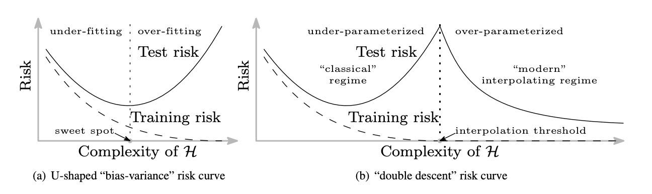
Modern models usually do not overfit per se, they usually converge like an "L-curve" (“modern interpolating regime” from this figure). Figure borrowed from here. -
Model complexity can be measured by: (i) the number of parameters (model size) for models with similar architectures, (ii) FLOPs, and (iii) the wall time on some given hardware. Model capacity is usually some function of model complexity. Big models usually take disproportionately more time to train. More complex layers are usually harder to train. Therefore it is better to favour standard well-tested modules with plain parallelizable architectures;
-
To test data augmentations, we usually design our pipeline so that there is only one parameter ranging from 0 to 1 that changes the extent of said augmentations. It becomes quite easy - you just need to run 3 experiments with this parameter equal to 0.2 / 0.5 / 0.9. Surprisingly, this approach is very similar to a fresh paper from Google;
-
Running full hyper-param sweeps may be prohibitively expensive, so
we only change significant params that amount to major changes in the logic or provide desired features. Additionally, we group similar changes together (i.e. "add more augmentations"), and first optimize the network to be faster and more compact and only then add more complexity. This “first minimize then add more complexity” assumption may not hold, but the sheer success of modern mobile architectures like MobilNet / EfficientNet / FBNet (to name a few) provides some assurance; -
Also, there are 2 nice principles often overlooked by ML researchers. One, Occam's Razor: if we do not know what a module does and what its properties are we do not use it. Ceteris paribus: if you change only one thing in your pipeline, most likely, there is no need to re-run the whole training process from scratch till full convergence. Most likely (unless you make drastic changes), you can make assumptions about convergence based on previous runs;
-
So, to find a better model, you need to build (or find) a good pipeline, fully fit your pipeline a couple of times and then start introducing small changes. Once in 10 or 20 runs, when you have added too many features, ablation runs or full runs until convergence may be warranted;
All of the below illustrations follow the same methodology:
-
All of the illustrations are mostly ceteris paribus, i.e. all other things are being held equal;
-
In particular, the train and validation datasets are the same, the ardware is the same, and most hyper-parameters are the same;
-
The validation dataset is the Open STT v0.5-beta validation dataset;
-
Though some of the changes are explicitly targeted at improving performance, all runs are executed at reasonably high hardware utilization (no IO bottle-necks, data feeding time close to zero, etc.).
-
We recorded the baseline runs (i.e. GRU models from Deep Speech PyTorch), but the datasets we used were vastly different (in our case our dataset also evolved drastically).
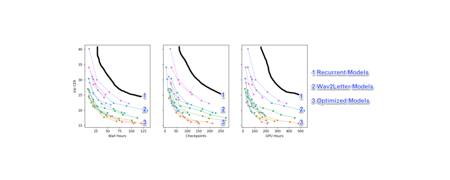
Overall Progress Made
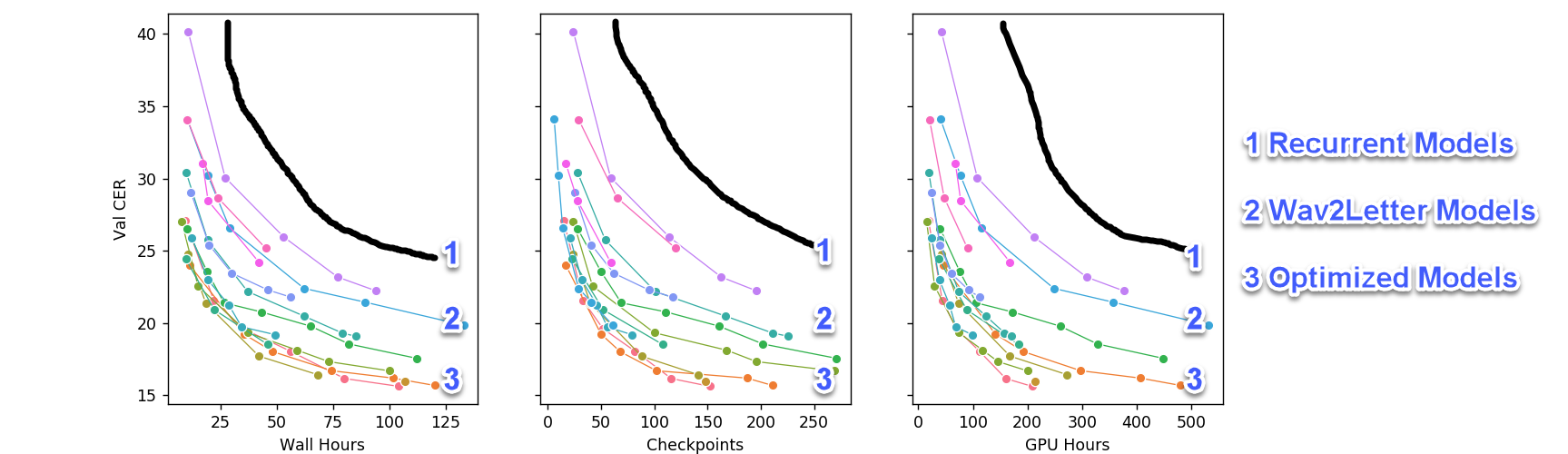
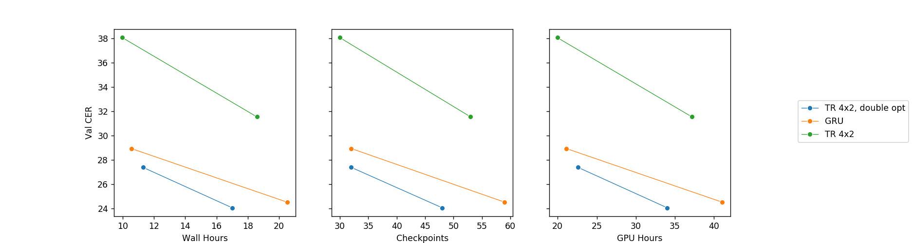
Initially we started with a fork of Deep Speech 2 in PyTorch. The original Deep Speech 2 model is based on a deep LSTM or GRU recurrent network, which are slow. The above image illustrates the optimizations we were able to add to the original pipeline. More specifically, we were able to do the following without hurting model performance:
- Reduce the model size around 5x;
- Speed up its convergence 5-10x;
- The small (25M-35M params) final model can be trained on 2x1080 Ti GPUs instead of 4;
- The large model still requires 4x1080 Ti but has a bit lower final CER (1 - 1.5 percentage point lower) compared to the small model.
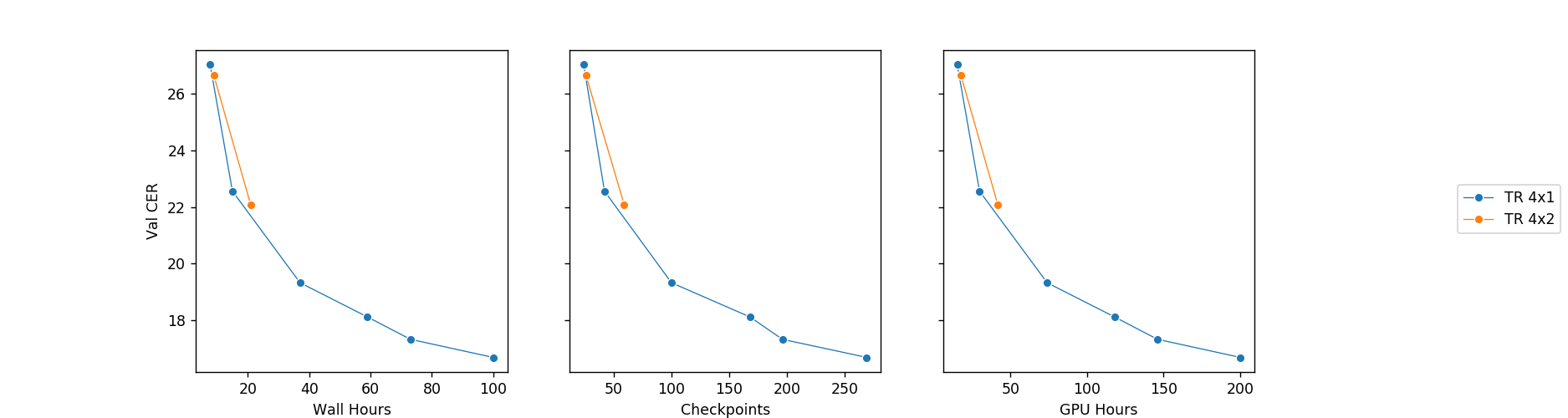
The above chart only has convolutional models, which we found to be much faster than their recurrent counterparts. We started on the process to getting these results as follows:
- Used an existing implementation of Deep Speech 2;
- Run a few experiments on LibriSpeech, where we noticed that RNN models are typically very slow compared to their convolutional counterparts;
- Added a plain Wav2Letter inspired model, which was actually underparameterized for Russian, so we increased the model size;
- Noticed that the model was okay, but very slow to train, so we tried to optimize the training time.
So, we then explored the following ideas to improve things:
Idea 1 - Model Stride
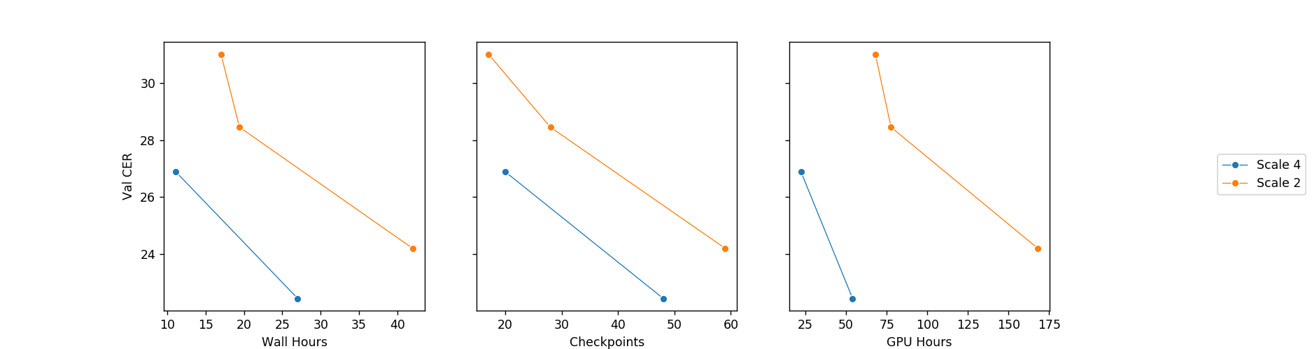
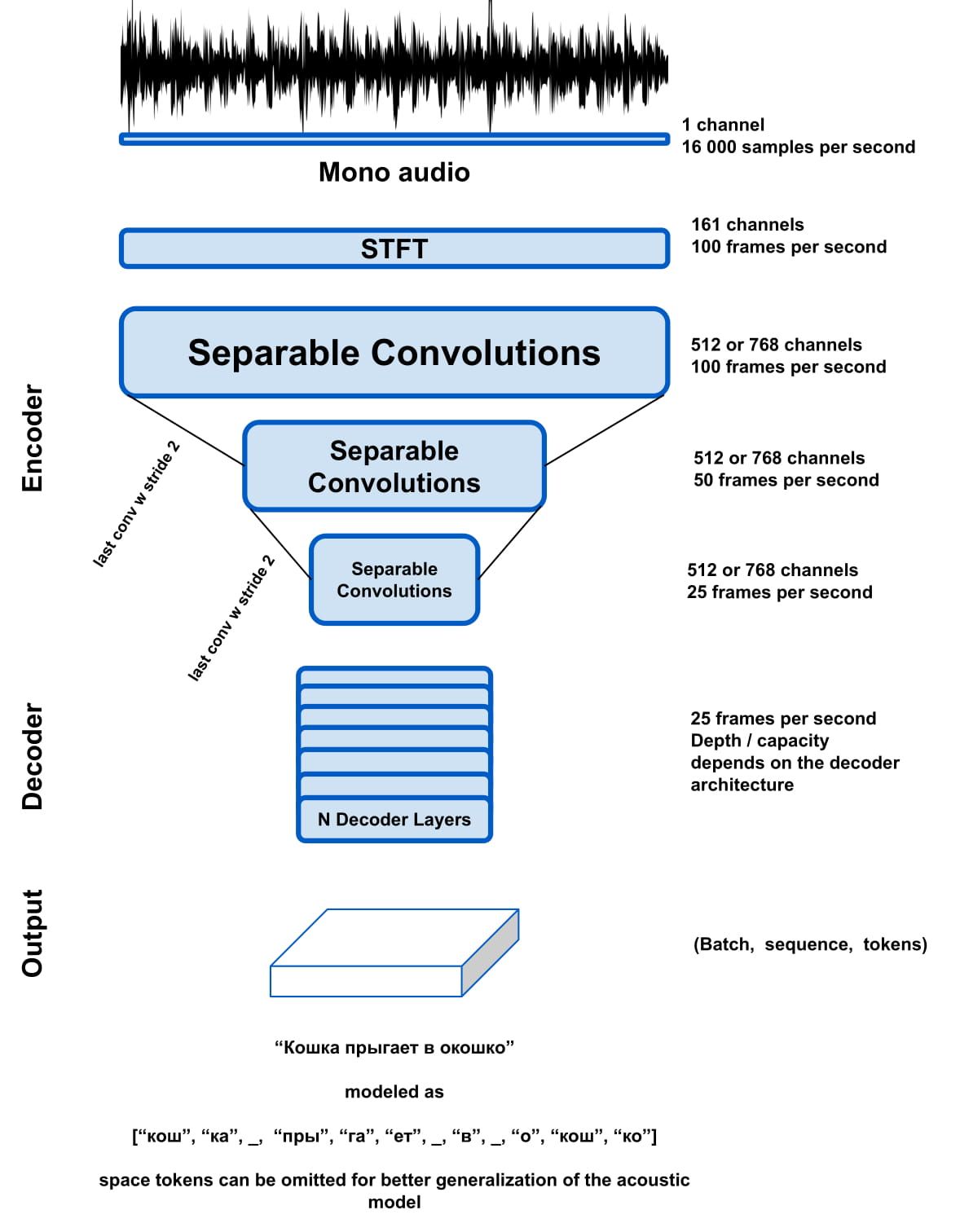
We started off our optimizations by first modifying the model stride. This is actually a very simple idea. When analyzing the output of a scaled-up version of Wav2Letter model with a stride of 2 (after Short-time Fourier transform), we noticed that the ratio of useful output tokens to blank tokens is roughly between 2:1 and 3:1. So, why not just add more stride within the convolutional encoder?
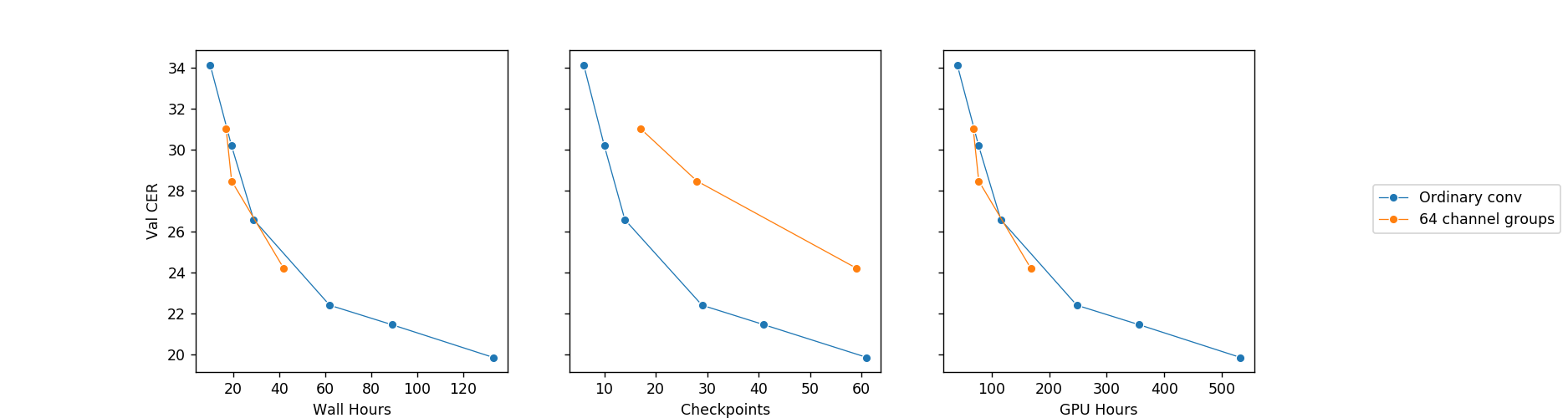
Idea 2 - Compact Regularized Networks
As mentioned above, the networks heavily optimized for mobile devices may not serve as an ideal source of architecture decisions, but the first generations of such networks provide excellent ideas:
-
Using separable > convolutions > as they drastically reduce the number of parameters in the models > without sacrificing performance;
-
Adding skip-connections to deep CNNs (first pioneered by > ResNets) because they speed up > convergence and allow you to train deeper models;
-
Adding attention modules like Concurrent Spatial and Channel > Squeeze & Excitation modules > or Style-based Recalibration > Modules in the convolutional > part of the model because they usually improve performance of the > model by adding a negligible computational overhead;
As an additional bonus, small regularized networks are easier to train because they overfit less. On the negative side, it takes more iterations for smaller networks to converge (in the sense that you can get through each batch faster, but you need more batches). It may be more complicated than that, but in our experience a simple rule of thumb says that if the network has 3-4x less weights, with all other things equal, it would take 3-4x more training steps to train to the same level of performance as the larger network. However, a smaller network will be 2-3x faster[^8].
There is also a promising idea that if you use IdleBlocks, i.e. pass some of your convolutional channels through your model without any operations, you can build deeper, more expressive networks with 2x less parameters and larger receptive fields.
Idea 3 - Using Byte-Pair Encoding
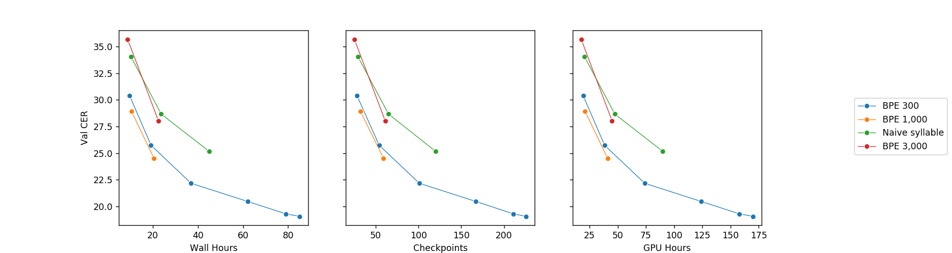
Compliant with the results of this paper we tried several tokenization approaches, and found that:
-
Byte-Pair Encoding (BPE) is a necessary condition to use a model > with overall stride larger than 4 - otherwise you just do not have > enough tokens;
-
Grapheme-based BPE works better than a phoneme-based BPE model;
-
In our case even a model with a very simple decoder started acting > as a language model of sorts, significantly reducing the WER > compared to baseline models. Keeping in mind that it is better to > do decoding using a separate model trained on larger text corpora, > we just made sure that our BPE models had similar or better CER > performance compared to baseline models;
-
The larger the BPE vocabulary the more the AM works like LM. It is > undesirable that the AM would overfit to known vocabulary, so a > balance needs to be found. We ran several models with different > BPE vocabulary sizes (300, 1,000, 3,000 and 10,000) and found out > empirically that using BPE token vocabulary up to 1,000 improves > acoustic model’s WER without hurting its CER. When we tried > vocabulary larger than 1,000 we started to see degradation in CER, > which we interpreted as the model had overfit to the vocabulary of > our spoken corpus;
We use the popular sentencepiece tokenizer with a small list of tweaks to fit the ASR domain.
Idea 4 - Better Encoder
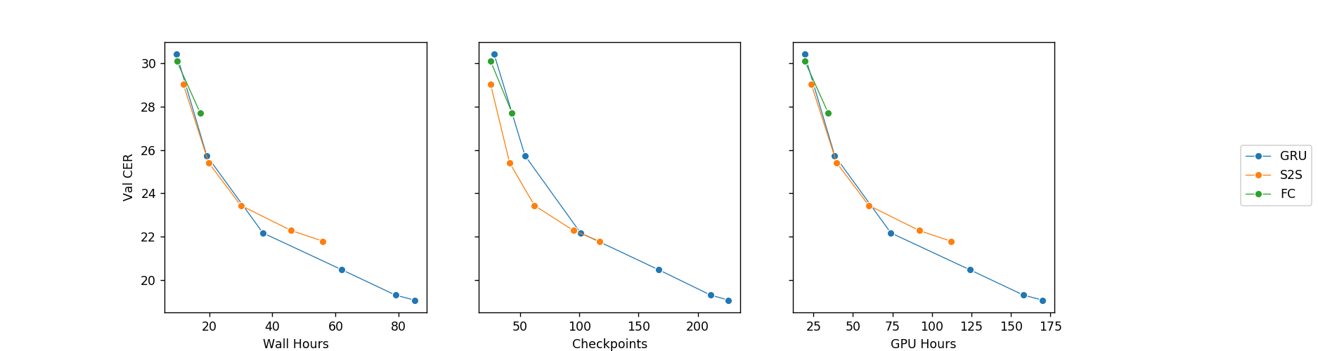
The basic idea here is to use a more expressive encoder-decoder architecture. The convolutional encoder with 8x down-scaling is very fast, so you can afford to use a much heavier decoder.
Though the wide-spread adoption of increasingly huge transformer models in NLP is debatable, the modelling capabilities of the transformer module are now widely accepted to be superior to previous state-of-the-art models.
Overall this setup produces models that are so computationally inexpensive, that you do not really need GPUs to deploy them in production. An acoustic model can easily run 500-1000 seconds of audio per GPU second (in practice this will be most likely bound by I/O) and 2-3 seconds of audio per CPU second (single processor core of a EX51-SSD-GPU server) without sacrificing performance. Note that this estimate includes only an acoustic model and further improvements can be obtained via model quantization and minification (i.e. pruning, teacher distillation, etc.).
Idea 5 - Balance Capacity - Never Use 4 GPUs Again
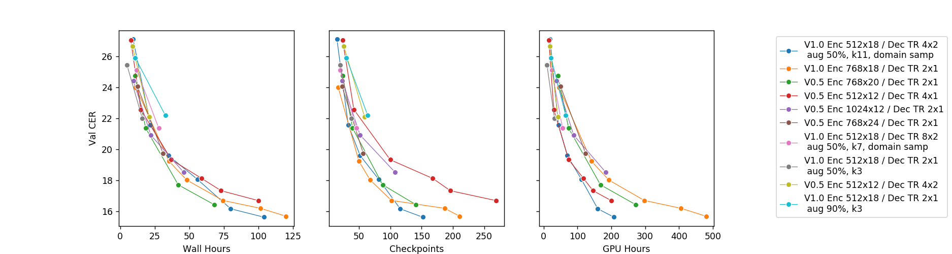
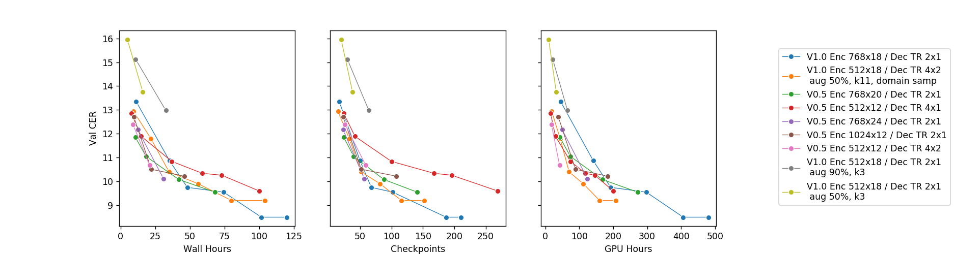
Overall, by balancing your capacity and compute in different parts of the model, you will get a model that quickly trains on only 2 1080 Tis (sic!) and achieves competitive results in days compared to models that might require 4 or even 8 GPUs.
I believe this is the most impressive achievement so far.
Idea 6 - Stabilize the Training in Different Domains, Balance Generalization
A big problem in speech is catastrophic forgetting. The root problem is that even regularized networks (with separable convolutions) start forgetting old domains when they are fit on mostly new data. This is especially undesirable for a production system. Another problem in speech is that ASR papers usually train 50 - 500 epochs on the full Librispeech dataset. This is highly sample inefficient and does not scale to real data.
We have found out that you can use curriculum learning to reduce the total number of steps required to fit a model on new data and deal with catastrophic forgetting with a few ideas. Using this approach we could reduce the total number of steps to under 5 - 10 * size of our dataset.
The key ideas are:
-
Use curriculum learning, i.e. sample data from your dataset > according to some quality metric (we used CER) such that you start > with the easier samples and gradually introduce more and more hard > examples as training progresses. In general it is undesirable to > sample too easy samples for too long (this will lead to > overfitting and poor robustness) or too difficult samples too > early (this will lead to underfitting). In our experiments we > found that maintaining 10% CER (by introducing harder or easier > samples as training progresses) is optimal;
-
When learning a new domain, sample additional data from the domains > you have trained on previously in order to reduce catastrophic > forgetting;
-
In real life, it is likely that the data from different domains is > heavily imbalanced. To counter this, you can sample data from your > domains with different probabilities to give your model the > required characteristics. For example, for the best models we just > assigned the same probabilities to all domains, but we defined our > domains to be sourced from similar sources (i.e. they have similar > noise, vocabulary, and topics)[^9].
-
Some domains may have higher or lower signal to noise ratio, so for > some domains optimal CER may be lowered to 5%;
Idea 7 - Make A Very Fast Decoder
This is out of scope for this article, but there are 2 options for post-processing:
-
A sequence-to-sequence network;
-
A beam search decoder with a language model;
In our tests, sequence-to-sequence networks do not visibly slow our inference whereas beam search is 10x slower. It is a point of further investigation to make a sequence-to-sequence model surpass beam search, but we were able to achieve a processing speed of around 25 seconds of audio per CPU core second using our implementation of beam search with KenLM without sacrificing its accuracy.
Model Benchmarks and Generalization Gap
In real life it is expected that if the model is trained on one domain, there will be a significant generalization gap on another. But is there a generalization gap in the first place? If there is, then what are the main differences between domains? Can you train one model to work fine on many reasonable domains with decent signal-to-noise ratio?
There is a generalization gap, and you can even deduce which ASR systems were trained on which domains. Also, with the ideas above, you can train a model that will perform decently even on unseen domains.
According to our observations, these are the main differences that cause the generalization gap between domains:
- Overall noise level;
- Vocabulary and pronunciation;
- The codecs or hardware used to compress audio;
| Dataset (hours) / out-of-dataset? | Our CER / WER | Best cloud CER / WER | Comment |
|---|---|---|---|
| Narration, yes | 3% / 11% | 3% / 6% | TTS narration dataset |
| AudioBooks, no | 9% / 30% | 7% / 25% | Very clean |
| YouTube, no | 15% / 37% | 16% / 32% | Very diverse |
| Radio, no | 8% / 19% | 14% / 26% | Very diverse |
| Public speech, no | 6% / 16% | 12% / 23% | Very diverse |
| Calls - taxi clean, yes | 7% / 20% | 7% / 15% | Clean annotation |
| Calls - e-commerce, yes | 19% / 34% | 17% / 31% | Noisy, rare words |
| Calls - pranks, yes | 22% / 43% | 23% / 39% | Very noisy |
Legend:
- All of the speed benchmarks were done on a EX51-SSD-GPU server - 4 core CPU + GTX1080;
- This benchmark includes both an acoustic model and a language model. The acoustic model is run on GPU, the results are accumulated, and then language model post-processing is run on multiple CPUs;
- The speed of the benchmark is measured by dividing the total audio duration of audio in the dataset by the total time spent applying acoustic model and language model post-processing. For these tests this metric ranged from 125 to 250, which is very fast, but bear in mind that this not representative of real production usage speeds;
More Detailed Benchmarks
The following figures are more detailed benchmarks of our solution vs. all the other major providers of Russian ASR. Note that the Narration and AudioBooks datasets are idealized domains, which means that high performance on the domain is not indicative of high performance in real life. The domains are roughly sorted in the order of their difficulty.
Some notes:
-
These results also include the language model post-processing and > mirror the table from the previous section;
-
Beam search uses a language model trained on a large external text > corpus;
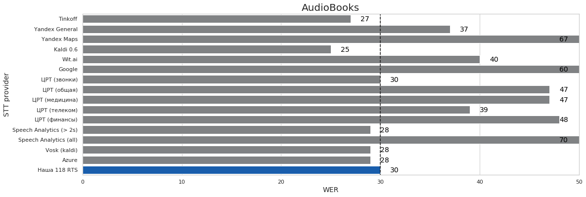
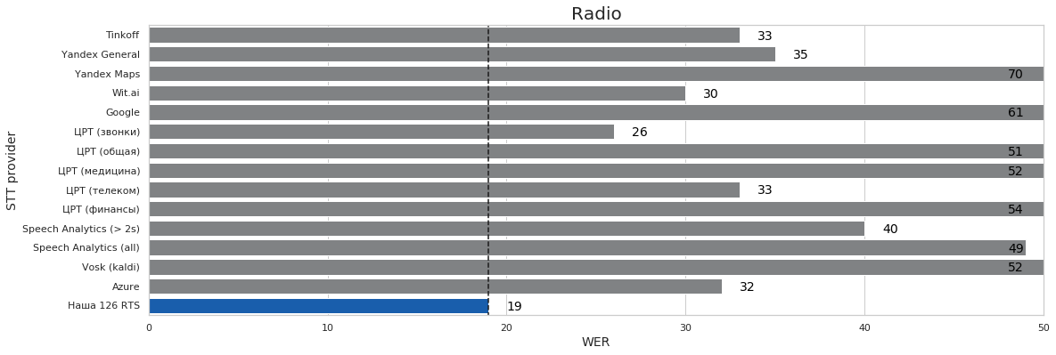
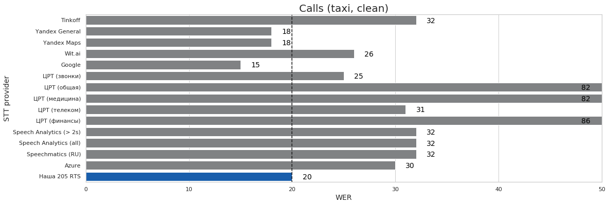
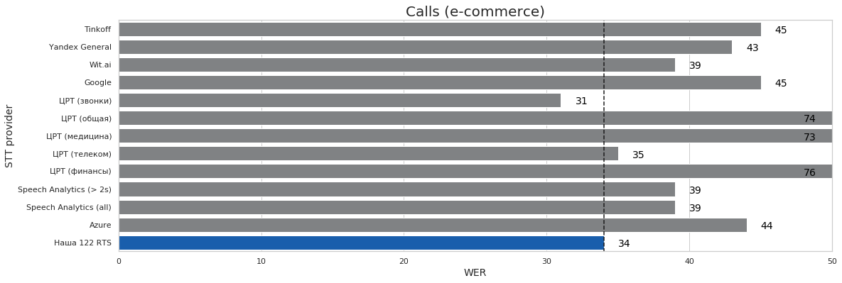
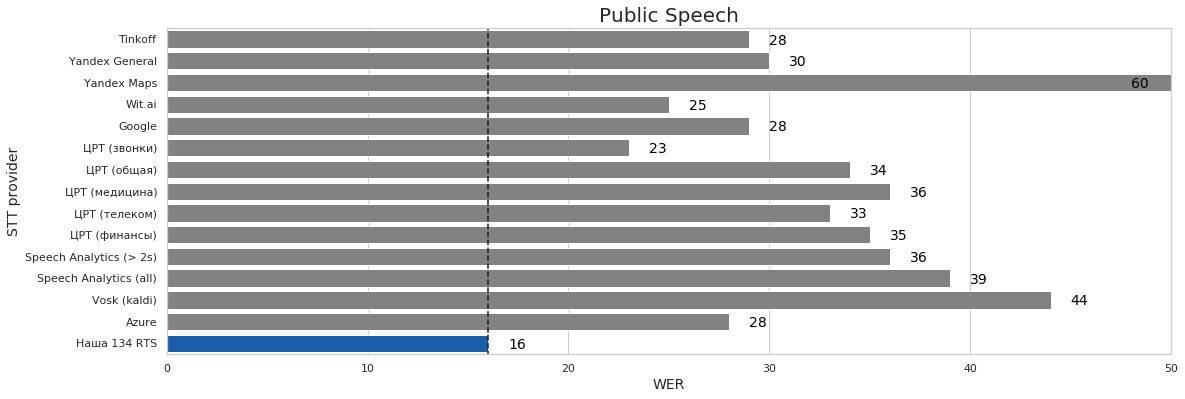
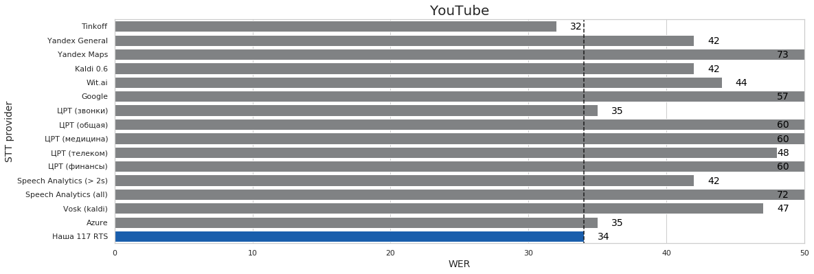
Model Benchmark Analysis
More often than not, when some systems are compared to other systems (if you speak Russian, this is a typical culprit) the following quirks occur:
- A new 2019 model is compared to a competitor's 2018 model;
- Results are cherry-picked to fit some narrative;
- Practical, compute, or maintenance concerns are omitted;
While we are not 100% immune to these deficiencies, we nevertheless argue that you should at least attempt to:
- Do out-of-dataset (ood) validation;
- Do validation on clean and noisy data;
- Try to create a general model suitable for real world usage. Obviously there is a reason why some companies provide several models for several domains, but creating a general model is more difficult than creating a model for a narrow domain;
- Compare the model to vastly different approaches - at least on a black box level;
Comparing the benchmarks in the previous section, some conclusions can be drawn (please note that these tests were made at the end of 2019 / early 2020):
- By using Open STT we managed to train a general model that performs on par with the best generalist models on the market and does not lag behind too much on out-of-dataset tests;
- No other model besides ours performs reasonably well on all of the validation sets without significantly sacrificing performance on some of the domains (i.e. WER > 50%);
- We can clearly see that for the majority of datasets for the majority of systems, there is a clear convergent performance of several best performing systems;
- Surprisingly, even though Google shows the best results on real calls, it severely lags behind on some of the domains. We could not understand whether it happened because of some arbitrarily high internal confidence threshold, but from the data it seemed that Google's STT just omits the output when it is not certain, which is less than desirable for some applications and the default behavior for others;
- Kaldi was probably trained on audio books or a similar domain;
- Even though on easy domains (such as narration or audio books) Tinkoff's models blow everybody out of the water, the performance on other domains is even worse than our models without LMs. Also they most likely trained their model on audio books and Youtube (or possibly narration or short commands);
- Surprisingly, despite the popular misconception, Yandex is not the best on the market for all domains;
- Though performing well on easier domains’ simple vocabulary, Kaldi falls behind on noisier domains.
Production Usage
We have shown that with close to zero manual annotation and a limited hardware budget (2-4 x 1080 Ti) you can train a robust and scalable acoustic model. But an obvious question is - how much more data, compute and effort is required to make this model deployable? How well does the model have to perform?
As for performance, an obvious criterion for us would be to beat Google on all of our validation datasets. But the problem with that is that Google has stellar performance on some domains (i.e. calls) and average performance on the others. Therefore for this section we decided to take the results of the best model of a local Russian state-backed monopoly SpeechPro that is usually cited as “the best” solution on the market.
| WER, our model | WER, our model, more capacity, more data |
WER, SpeechPro Calls | |
|---|---|---|---|
| Narration | 11% | 10% | 15% |
| AudioBooks | 30% | 28% | 30% |
| YouTube | 37% | 32% | 35% |
| Radio | 19% | 19% | 26% |
| Public speech | 16% | 16% | 23% |
| Calls taxi (clean) | 20% | 14% | 25% |
| Calls e-commerce | 34% | 33% | 31% |
Looking at the above table, we found that our model outperforms SpeechPro Calls (they have many models, but only this one performs well on all of the domains) for all categories except for e-commerce calls and audiobooks. Additionally, we found that adding more capacity to the model and training on more data greatly improved our results for most domains, and that SpeechPro only outperforms this model on e-commerce calls.
To achieve these results we had to source an additional 100 hours of calls with manual annotation, around 300 hours of calls with various sources of automatic annotation and 10,000 hours of data similar to OpenSTT, but not yet public. We also had to increase the model decoder capacity by bumping its total size to around 65M parameters. If you speak Russian, you can test our model here.
As for other questions, it is a bit more complicated. Obviously you need a language model and a post-processing pipeline, which is not discussed here. To deploy on just CPU some further minification or quantization is desirable but unnecessary. Being able to process 2-3 seconds of audio per CPU core second (on a slow processor, on faster processor cores we get somewhere around 4-5) is good enough, but state-of-the art solutions claim figures around 8-10 seconds (on a faster processor).
Further Work
Here is a list of ideas, that we tested (some of which even worked), but we decided in the end that their complexity does not justify the benefits they provide:
- Getting rid of gradient clipping. Gradient clipping takes from 25% to 40% of batch time. We tried various hacks to get rid of it, but could not do it without suffering a severe drop in convergence speed;
- ADAM, Novograd and other new and promising optimizers. In our experience, they worked only with simpler non speech related domains or toy datasets;
- Sequence-to-sequence decoder, double supervision. These ideas work. Attention-based decoders with categorical cross-entropy loss instead of CTC are notoriously slow starters (you add speech decoding to the already burdensome task of alignment). Hybrid networks did not perform much better to justify their complexity. This probably just means that hybrid networks require a lot of parameter fine-tuning;
- Phoneme-based and phoneme-augmented methods. Though these helped us regularize a few over-parametrized models (100 - 150M params), they proved not very useful for smaller models. Surprisingly an extensive tokenization study by Google arrived at the similar result;
- Networks that increase in width gradually. A common design pattern in computer vision, so far such networks converged worse that their counterparts with the same network width;
- Usage of IdleBlocks. At first glance, this did not work, but maybe more time was needed to make it work;
- Try any sort of tunable filters instead of STFT. We tried various implementations of tunable STFT filters and SincNet filters, but in most cases we could not even stabilize the training of the models with such filters;
- Train a pyramid-shaped model with different strides. We failed to achieve any improvement here;
- Use model distillation and quantization to speed up inference. At the moment when we tried native quantization in PyTorch it was still in beta and did not support our modules yet;
- Add complementary objectives like speaker diarization or noise cancelling. Noise cancelling works, but it proved to be more of an aesthetic use;
References
References ==============
Github Repos and Datasets =============================
-
Open STT dataset (*)
-
Sentencepiece toolkit for > byte-pair-encoding
Articles, Blogs, and Web Resources --------------------------------------
-
Proper STT system quality > benchmarks > in English (*)
-
CTC loss (*)
Papers ----------
Computer Vision Papers
Speech To Text Papers
Author Bio
Alexander Veysov is a Data Scientist in Silero, a small company building NLP / Speech / CV enabled products, and author of Open STT - probably the largest public Russian spoken corpus (we are planning to add more languages). Silero has recently shipped its own Russian STT engine. Previously he worked in a then Moscow-based VC firm and Ponominalu.ru, a ticketing startup acquired by MTS (major Russian TelCo). He received his BA and MA in Economics in Moscow State University for International Relations (MGIMO). You can follow his channel in telegram (@snakers41).
Acknowledgments
Thanks to Andrey Kurenkov and Jacob Anderson for their contributions to this piece.
Citation
For attribution in academic contexts or books, please cite this work as
Alexander Veysov, "Toward's an ImageNet Moment for Speech-to-Text", The Gradient, 2020.
BibTeX citation:
@article{veysov2020towardimagenetstt,
author = {Veysov, Alexander},
title = {Toward's an ImageNet Moment for Speech-to-Text},
journal = {The Gradient},
year = {2020},
howpublished = {\url{https://thegradient.pub/towards-an-imagenet-moment-for-speech-to-text/ } },
}
If you enjoyed this piece and want to hear more, subscribe to the Gradient and follow us on Twitter.

